To discover unexplored data and information in the deep-sea for future research, deep-sea exploration has become the commanding height of international competition. In the process of deep-sea exploration, visual information plays a significant role in a series of activities, such as navigation^[1-3], object recognition^[4-6] and underwater robotics^[7]. However, the imaging quality always severely degrades when meeting marine snow or when the sediment particles on the seabed are stirred up by a robotic arm or a landing Autonomous Underwater Vehicle (AUV). Caused by the scattering of tiny particles in the turbid water body, this phenomenon may bring obstacles or even dangers to deep-sea exploration. Therefore, it is of great importance to remove scattering effect and see targets clearly through turbid water in the deep-sea.

Existing underwater descattering methods can be mainly classified into the model-free and model-based methods. The model-free algorithms directly enhance image contrast without considering the physical scattering mechanisms. For example, contrast limited adaptive histogram equalization (CLAHE)^[8] improves the image contrast in a local manner. Retinex theory^[9] separates an image into illumination and reflectance components, and then estimates both of them. Generalized unsharp masking (GUM)^[10] improves contrast and sharpness of the image while reducing the halo-effect. Besides, the fusion-based method^[11-13] combines white-balanced and contrast-enhanced images derived from an original image. However, these algorithms do not model the image degradation process caused by scattering, which may fail in some extremely scattering situations. Among the model-based methods, dark channel prior (DCP)^[14] based on simplified Jaffe-McGlamery model^[15] in which scattering is decomposed into the respective effects of atmospheric illumination and transmission map to descatter. To extend DCP into underwater, underwater dark channel prior (UDCP)^[16] considers selective absorption of different wavelength underwater, thus more refined transmission map estimation results are obtained to better improve image quality. UDCP is unsuitable for deep-sea situations, because it supposes that atmospheric illumination is uniform, while in the deep-sea, atmospheric illumination almost comes from artificial light and inevitably causes non-uniform illumination. Peplography^[17] models and estimates scattering as a veiled image with a Gaussian distribution. However, Peplography supposes that targets to be observed is from the same depth, which is not often the case in the deep-sea.

Overall, existing methods are limited in deep-sea scattering environment with multi-depth or non-uniform illumination. In this paper, we propose a deep-sea descattering method based on a depth-rectified statistical scattering model. To deal with multi-depth scenarios, the transmission map is utilized to rectify the scattered light emitted by different scene depths. To cope with non-uniform illumination, a depth-rectified scattering map is calculated locally in each color channel with a Gaussian statistical scattering model, representing the spatial distribution of the scattered light in the RGB color channels, which can remove the scattering map from the input image. Experimental results for different underwater images and videos captured in shallow and deep-sea show that the proposed method outperforms the existing methods in terms of subjective quality and objective evaluation. The rest of the paper is organized as follows. The proposed method is introduced in Section 2. The experimental settings and results are shown in Section 3. Finally, conclusions are drawn and discussed in Section 4.

Because of the deficiency of sunlight in the deep-sea, artificial illumination needs to be introduced for better observation. However, this will bring non-uniform illumination as shown in Fig.1, which is different from the situation in the shallow sea.

Figure 1.  Non-uniform illumination and multi-depth scenarios in deep-sea

Traditional Gaussian statistical scattering model^[17] supposes that the targets to be observed locate at the same depth. However, many deep-sea scenarios, shown in Fig.1, do not satisfy this assumption since the camera shooting angle is not always perpendicular to the seabed and the objects are always at different depths, so the ratio of the scattered light will increase with depth.

The overall framework of the proposed deep-sea descattering method is provided in Fig.2. Firstly, we use the transmission map to rectify the scattered light emitted by different depths. Then, a depth-rectified scattering map is calculated in the RGB color channels separately with a Gaussian statistical scattering model to represent the spatial distribution of the scattered light. Finally, the descattering image is obtained after removing the scattering map from the input image.

Figure 2.  Overall framework of the proposed deep-sea descattering method

First, considering that scattered light exhibits nonlinear enhancement with distance, we utilize the transmission map which reflects the attenuation ratio of ballistic light at different scene depths, corresponding to the inverse of the enhancement ratio of the scattered light. In order to estimate the transmission map t, we compare several methods and finally choose the underwater dark channel prior (UDCP)^[16] which considers selective absorption underwater to estimate the transmission map t.

To deal with multi-depth scenarios, the transmission map is utilized to model the depth-constant scattered image. we multiply the input image $ I $ with transmission map t pixel by pixel to obtain a depth-constant scattered image $ {I}^{norm} $ with the scene depth restrained to be the same, which can be expressed as

where i and j are the pixel coordinates of $ {I}^{norm} $.

The resulting image $ {I}^{norm} $ meets the depth-constant assumption of the Gaussian statistical scattering model^[17], so, a scattering map can be correctly estimated by the model to represent the spatial distribution of the scattered light, and in order to cope with non-uniform illumination, we calculate the depth-rectified scattering map locally. Based on this, the scattering in a window $ {X}_{ij} $ with the size of $ {w}_{x}\times {w}_{y} $ is considered to have a mean value of $ {\mu }_{ij} $ and the variance of Gaussian distribution of $ {\sigma }_{ij} $:

where $ {X}_{ij} $ is the ith column and jth row local area of $ {I}^{norm} $, m and n are the coordinates in the window $ {X}_{ij} $, and N_x, N_y are the total number of pixels in the x and y directions of $ {I}^{norm} $, respectively.

Here, the maximum likelihood estimation (MLE) is used to estimate the mean value of the unknown parameter $ {\mu }_{ij} $ by calculating the mean value of the pixels in the window $ {X}_{ij} $:

where $ {\widehat{\mu }}_{ij}^{norm} $ is the estimated sample mean of the local area ($ {w}_{x}\times {w}_{y} $), $ L\left(\cdot \right) $ is a likelihood function of Gaussian distribution, $ {X}_{ij} $ are the random variables, $ {x}_{ij} $ is a cropped window area, and $ {\stackrel{̄}{x}}_{ij} $ is mean value of the cropped window area.

Further, to compensate the depth information that is lost in $ {I}^{norm} $, the actual scatter map of $ \widehat{\mu } $ of the input image $ I $ is obtained by dividing the scatter map $ {\widehat{\mu }}^{norm} $ by the transmission map t:

Then, the descattering image $ {I}^{'} $ is calculated by subtracting the actual scatter map $ \widehat{\mu } $ from the input image I:

There are some excessive and dark pixels in the descattering image, so we select the brightest and the darkest pixels to limit them, and then normalize the image to obtain the output image. Note that all the above operations are applied on RGB color channels of the input image, respectively.

Further, we discuss the impact on the proposed algorithm in the case of non-uniform illumination. The used transmission map $ t $ is calculated based on the UDCP, so the transmission map $ t $ can be written as

where A is the global illumination, $ {I}^{dark} $ is the dark channel image of the input image I.

Substituting Eq.(6) into Eq.(1) we can get

Based on Eq.(3) and Eq.(7), we can calculate

where $ E\left(\cdot \right) $ is the expectation operator.

Finally, by combining Eq.(1), (4), (5), (7) and (8) together, we can calculate that

According to the derivation results, we found that the global illumination term A significantly affects the quality of transmission map. Because of multiple searchlights in the deep-sea probe, the global illumination of the image is non-uniform. However, in a local area, the illumination can be considered to be approximately equal, which means that the light is uniform in this area. The proposed method takes a regional processing, thus the global illumination term A of Eq.(9) in a block can be regarded as constant, so the algorithm is effective when the illumination in the block is uniform.

In this section, in order to demonstrate the effectiveness of the proposed method, the performance of the proposed method is compared with seven existing methods: DCP^[14], a representative descatter method based on the assumption that the darkest channel of RGB retains the effective information of the image; UDCP^[16], which considered the selective absorption of different wavelength underwater; GUM^[10], improved the image quality by extracting and amplifying the high frequency part of the image; Fusion method^[8], which processed a single image differently, and then merged the obtained multiple images to obtain a result with better imaging quality; Retinex^[9], based on the human visual system to performs color correction and contrast enhancement on images; Peplography^[17], improved image quality by assuming that scattering satisfies Gaussian distribution; CLAHE^[8], enhanced the bright areas and attenuating the dark areas to enhanced the overall contrast of the image.

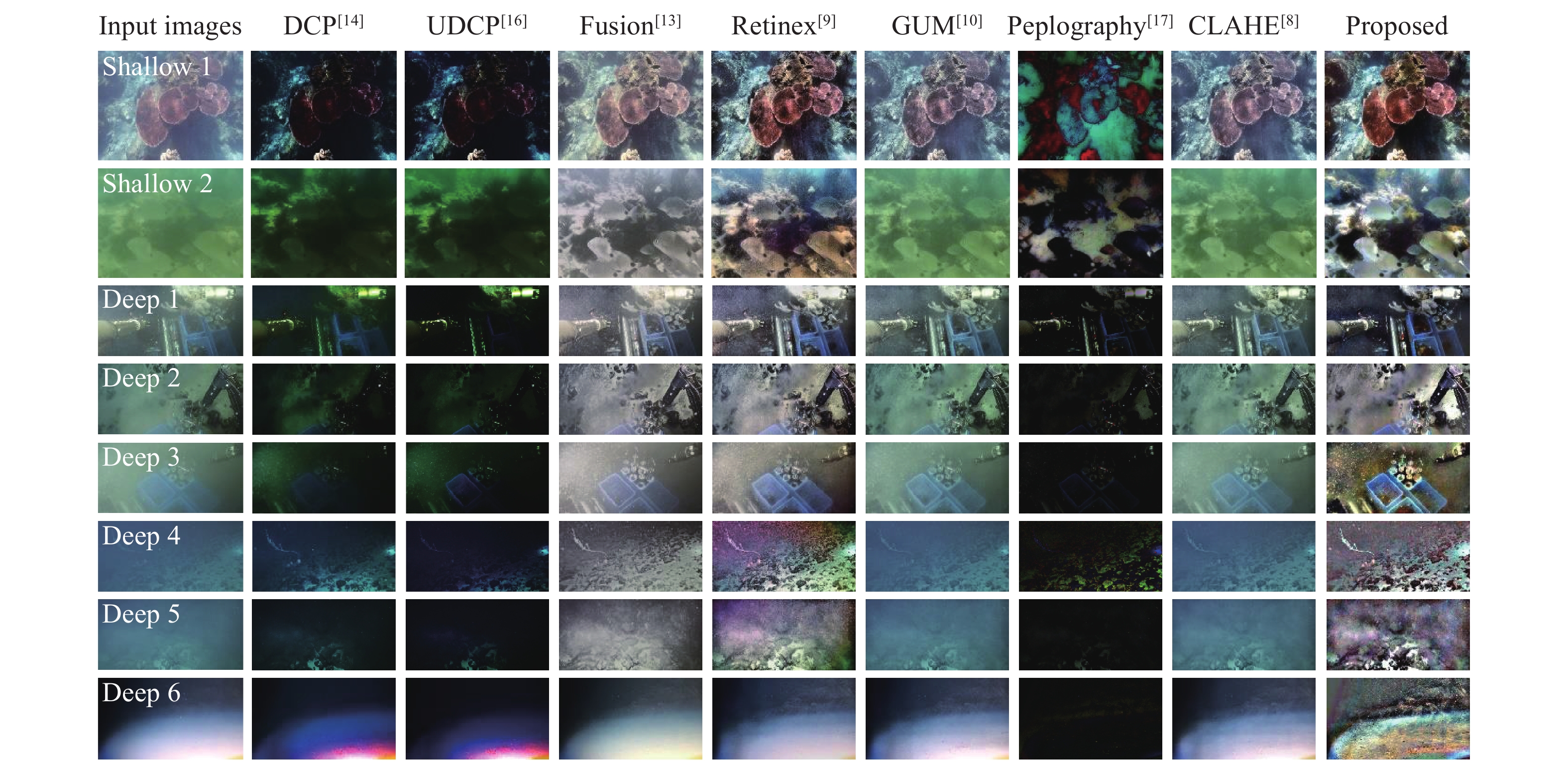
The experiments are conducted on scattering images/videos captured in the shallow sea and deep-sea. The data of shallow sea are from UIEB^[18] dataset. The deep-sea videos was collected by Deep Sea Video Technology Laboratory, Institute of Deep-sea Science and Engineering, Chinese Academy of Sciences in the South China Sea with the self-developed deep-sea imaging and recording system "Lan Mou" equipped with deep-sea high resolution stereo camera and deep-sea LED illumination. The parameters and the features of the images and videos are listed in Tab.1 with sample frames. The shallow sea data contains image with color shift and scattering. In order to verify that the proposed algorithm can deal with the scattering in the shallow sea, and can have a better visual presentation effect. The data of the deep-sea are video sequences, including strong and weak scattering; the scattering is relatively stable and dynamic; the illumination is relatively uniform and the illumination is non-uniform. By selecting these data, the effectiveness and robustness of the proposed algorithm can be verified. The images in Fig.3 are the 270^th, 241^st, 61^st, 50^th, 1^st and 7^th frame in the corresponding videos.

Table 1.  Overview about 2 images and 6 video sequences

Video sequence	Frame rate	Resolution	Frame number	Contents	Scattering intensity	Sample images
Shallow 1	1 fps	640×480	1	Coral	+
Shallow 2	1 fps	640×480	1	Fish	+
Deep 1	30 fps	1 920×930	300	Robot arm and acquisition equipments	+++
Deep 2	30 fps	1 920×930	1 080	Robot arm and acquisition equipments	++
Deep 3	30 fps	1 920×930	750	Robot arm and acquisition equipments	++++
Deep 4	30 fps	1 920×930	450	Seabed and plant	+
Deep 5	30 fps	1 920×930	420	Seabed	++++
Deep 6	30 fps	3 840×2 160	330	Seabed	+

Figure 3.  Subjective comparisons on shallow sea and deep-sea images. From left to right are input underwater images, and the results of DCP^[14], UDCP^[16], Fusion^[13], Retinex^[9], GUM^[10], Peplography^[17], CLAHE^[8], and the proposed method

For the shallow sea images shown in Fig.3, the results of DCP, UDCP, GUM, Peplography and CLAHE in descattering and improving image visibility are unsatisfactory. Fusion and Retinex are more robust and effective than DCP, UDCP, GUM, Peplography and CLAHE, but they still do not remove the scattering well, and there is still a scattering mask on the result. Our method produces images with high visibility, well descattering and clear detail.

For the deep-sea images shown in Fig.3, the results of DCP, UDCP, GUM, Peplography and CLAHE in enhancing the contrast and descattering is poor, and DCP, UDCP, and Peplography will introduce a larger color cast. Although Fusion and Retinex remove the color cast to a certain extent, which improves the visual effect of the picture, they do not effectively remove the scattering. Our method significantly removes the effects of scatter and improves the visual effect of the images. In addition, our method also shows good performance when the scattering is non-uniform.

Furthermore, we select underwater color image quality evaluation metric (UCIQE)^[19] which is an evaluation index of underwater image quality. UCIQE is a linear combination of chroma, saturation and contrast, which is an important indicator of underwater image quality evaluation. UCIQE can be defined as UCIQE = c₁ × σ_c + c₂ × con_l +c₃ × μ_s, where σ_c is the standard deviation of chroma, con_l is the contrast of luminance, and μ_s is the average of saturation. And, c₁ = 0.4859, c₂ = 0.2745 and c₃ = 0.2576 in Ref. [19].

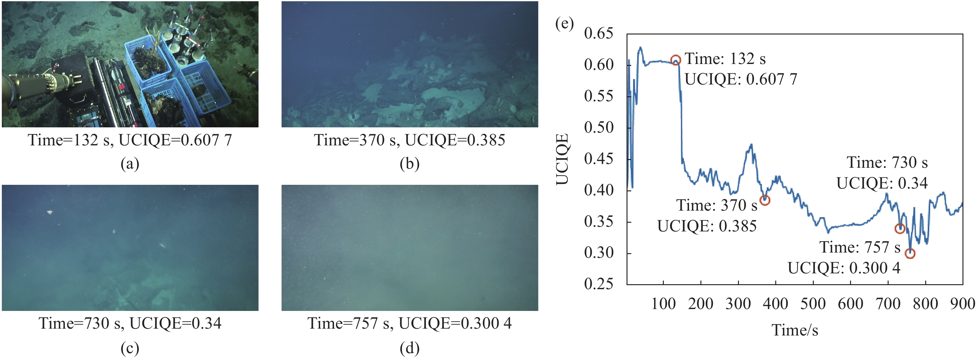
The proposed method aims to process the videos or images directly, so that it can be applied to data in any shooting scene. However, due to the lack of the measured scattering intensity during video shooting, the evaluation value of the image domain is used to describe the scattering intensity. The research found that there is a positive correlation between UCIQE and the subjectively visible scattering intensity^[19], so we have marked the UCIQE value for each set of test data to represent the variation of the scattering intensity.

In Fig.4, we calculate the UCIQE of the deep-sea video, and obtain the UCIQE value of the video at different times, and we present some video frames with different UCIQE values. It is found that the smaller the UCIQE value, the larger the scatttering intensity of the image, and vice versa.

Figure 4.  Objective comparisons of deep-sea video. (a)-(d) are the video frame samples in the video and their UCIQE values; (e) is the UCIQE results of the video

We also use UCIQE to evaluate the result of image reconstruction quality of underwater images shown in Fig.3. Table 2 gives the evaluation scores of these methods applied to shallow sea and deep-sea images shown in Fig.3. In both of deep-sea and shallow sea, the proposed method has a higher UCIQE value than other methods, reflecting the universality, efficiency and robustness of proposed algorithm.

In order to verify the effectiveness and robustness of the algorithm in dynamic scattering scenarios, we also tested the deep-sea scattering videos, and used UCIQE as an evaluation indicator, the average UCIQE of the video sequences were shown in Tab.3 and the UCIQE results of the video sequences were shown in Fig.5.

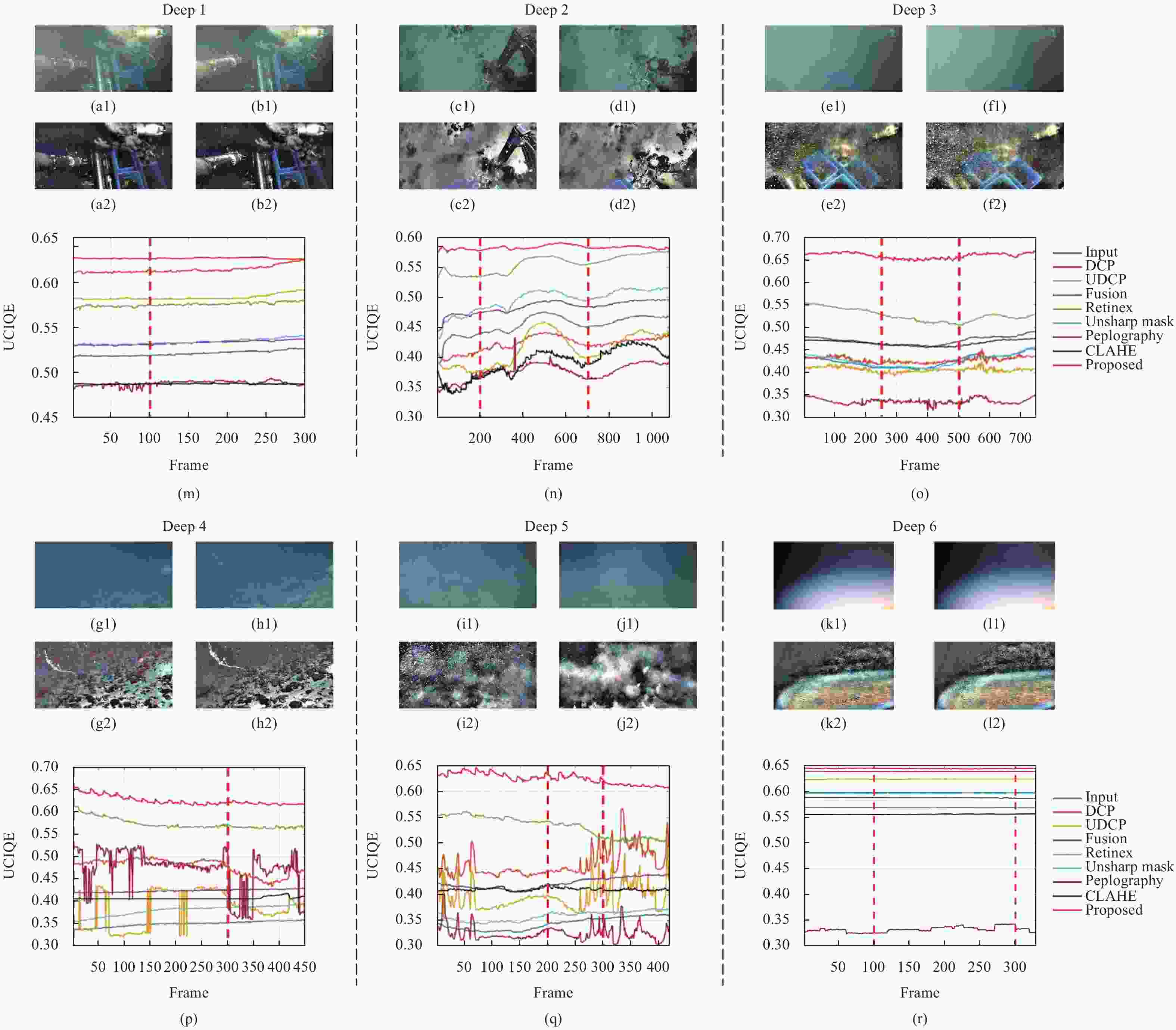
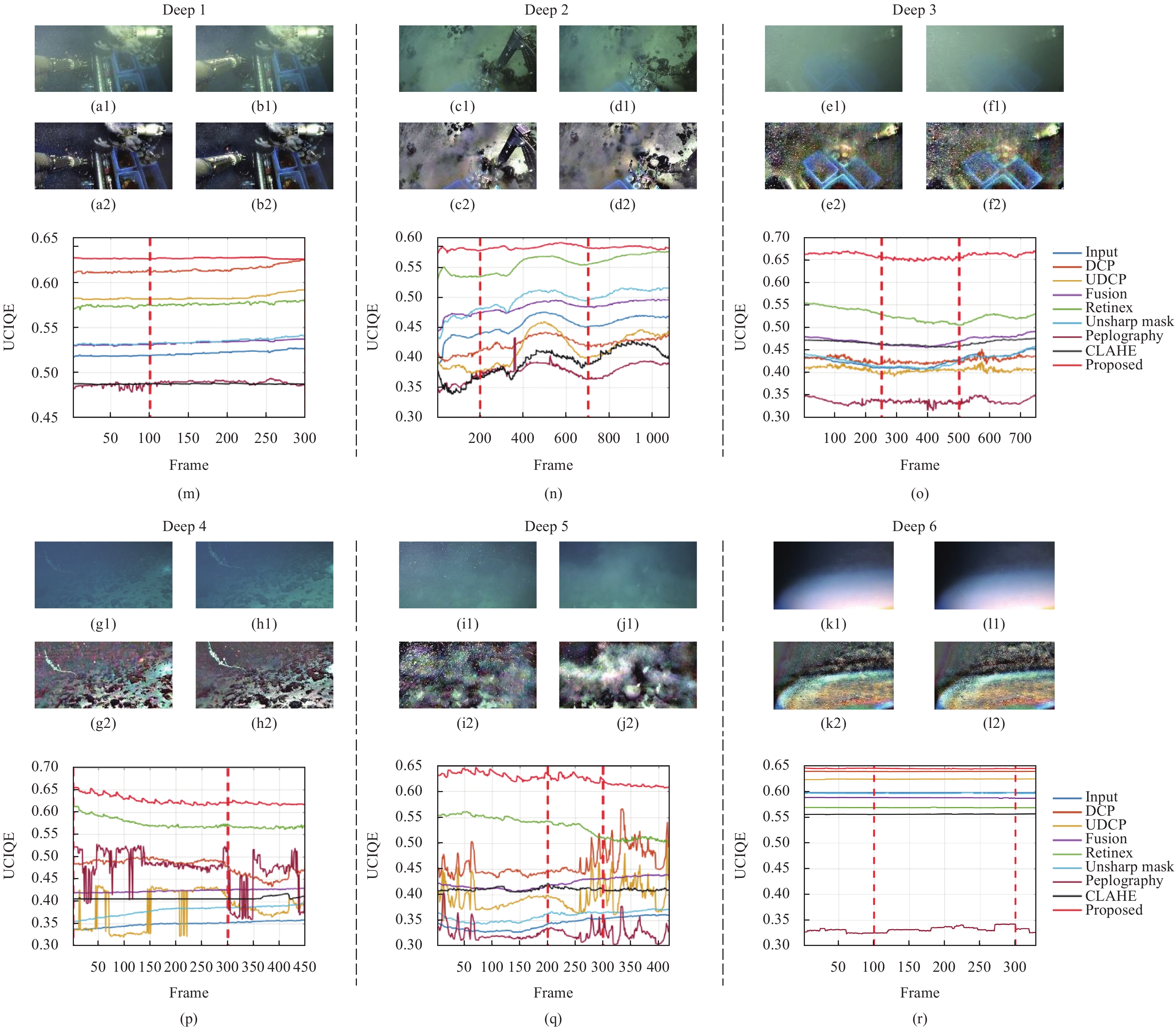
Figure 5.  Objective comparisons of six deep-sea videos corresponding to Deep 1-6. (a1) to (l1) are the video frame samples in the six videos; (a2)-(l2) are the results of (a1) to (l1) of the proposed algorithm; (m)-(r) are the UCIQE results of the six videos by different methods. The red dotted line in (m) to (r) mark the corresponding frame of the above video frame samples in (a1)-(l1)

In Tab.3, compared with other methods, our method can have higher UCIQE in different scenarios, which reflects the effectiveness of our algorithm. The scattering intensity is different between different videos, and our method can improve UCIQE by 8% to 79% on these data sets which reflecting the robustness of the algorithm.

In Fig.5(m), (o) and (r), it can be shown that when the scenes with little dynamic changes in scattering, the stability of the performance of all methods is well. The proposed method has a significantly higher UCIQE, and the performance is relatively stable throughout the video. In Fig.5(n), (p) and (q), it is shown that when the scenes with large dynamic changes in scattering, the UCIQE of existing methods fluctuates significantly, while that of the proposed method always has good stability. Moreover, UCIQE of the proposed method is much higher than those of other algorithms, which reflecting the effectiveness and robustness of our algorithm.

Here, we will discuss the physical limit of our proposed algorithm. We applied our proposed method to the images with different scattering intensities. The results are shown in Fig.6.

Figure 6.  Subjective and objective comparisons on deep-sea images with different scattering intensities from Haze 1 to Haze 5. From left to right are input underwater images, and the results of DCP^[14], UDCP^[16], Fusion^[13], Retinex^[9], GUM^[10], Peplography^[17], CLAHE^[8], and the proposed method

In Fig.6, the scattering of Haze1 to Haze 5 increased gradually. From the image Haze 2 (UCIQE=0.3705), we can find that DCP, UDCP, GUM, Peplography and CLAHE can no longer improve the image quality, while Fusion, Retinex and proposed algorithm can also effectively remove the scattering phenomenon. When the scattering intensity increases to Haze 4 (UCIQE=0.3442), the results reconstructed by Fusion and Retinex are more difficult to distinguish effective information, however, some information can be distinguished in the reconstruction results of proposed algorithm. When the scattering intensity reaches Haze 5 (UCIQE=0.3251), the effective information cannot be reconstructed by the proposed algorithm which is considered to reaches its physical limit in this case.

In this paper, to deal with multi-depth and non-uniform illumination in deep-sea scattering environment, we proposed a deep-sea descattering method based on a depth-rectified statistical model. First, in order to rectify the scattered light emitted by different scene depths, the transmission map is utilized. Then, in each RGB channel, we calculate a depth-rectified scattering map with a Gaussian statistical scattering model to represent the spatial distribution of the scattered light. Finally, after the scattering map subtraction from the input image, the descattering image is obtained. Experimental results with shallow and deep-sea images and videos demonstrate the efficiency and effectiveness of the proposed method compared the existing methods in terms of subjective quality and objective evaluation. In the future, we can improve the computational efficiency for the real-time requirements in actual scenes.

Thanks for the deep-sea data provided by Deep Sea Video Technology Laboratory, Institute of Deep-sea Science and Engineering, Chinese Academy of Sciences and the great support for this work.