

-
海洋上层物质具有明显的水平和垂直分布特征,影响着海洋生态系统的结构和功能。过去四十年间,人们利用被动海洋水色遥感技术估算天然水体的光学性质和悬浮粒子的分布,彻底改变了对海洋的认知。然而,被动探测技术无法在夜间进行,也会受到云层、气溶胶和太阳天顶角的影响,限制了其在获取海水粒子的形态和大小分布信息的能力。海洋激光雷达提供了一种测量上层海洋生物量垂直分布的技术,成为目前最有潜力的遥感手段;另外,激光雷达回波信号提供了关于海洋粒子散射的偏振信息,有助于研究海水粒子的物理和生理状态[1]。
多次散射效应是激光在海水中传输的一个复杂问题,也是光学深度较大的介质中的重要退偏来源。为了探究激光在海水中发生多次散射的辐射传输过程,需要建立合适的辐射传输模型[2]。蒙特卡洛模型是数值求解辐射传递方程常用的替代方法,能够模拟水中激光辐射传递过程。目前,在非偏振光方面,国内外很多研究机构已经建立了适用于多种介质的蒙特卡洛辐射传输模型,并实现了较多应用;在偏振光方面,利用偏振蒙特卡洛在探测水云[3-4]、水体[5-6]、生物组织[7]等方面取得了较多成果。但应用在海洋上的模型很少,利用该模型仿真水体垂直剖面的探测回波并对影响偏振测量误差主要因素的研究更少,因此有必要建立水中激光偏振辐射传输模型并分析不同光学参数的水体和激光雷达测量模式下的偏振测量误差。
文中使用高斯分布设置了三种深度均分布在10~30 m的低、中、高浓度散射层,其叶绿素a峰值浓度分别为0.1 mg/m3、1 mg/m3和10 mg/m3。通过建立偏振蒙特卡洛仿真模型研究发射波长为532 nm的船载偏振激光雷达水体垂直剖面的偏振探测回波,分析低、中、高浓度散射层水体和接收视场角为10~1000 mrad之间的偏振测量误差。
-
1852年,George Stokes介绍了一组用来描述偏振光辐射的参数,这组参数称为斯托克斯矢量。斯托克斯矢量能够量化光的偏振状态和由于散射过程而发生的偏振变化,用光强或辐射能量表示真实可观测的量,不仅能描述完全偏振光还可以描述非偏振光和部分偏振光,通常利用光电探测器、线性偏振器和圆偏振器进行测量。斯托克斯矢量中的四个参数分别是I、Q、U和V,其中I描述的是一束光的总能量,Q描述的是水平线偏振(Q = +1)或垂直线偏振(Q = −1)的量,U描述的是+45°线性偏振(U = +1)或−45°线性偏振(U = −1)的量,V描述的是右旋圆偏振(V = +1)或左旋圆偏振(V = −1)的量[8]。
斯托克斯矢量的旋转需要选取适当的参考坐标系,旋转矩阵R(ψ)表示如下[9]:
$$R(\psi ) = \left[ {\begin{array}{*{20}{c}} 1&0&0&0 \\ 0&{\cos 2\psi }&{\sin 2\psi }&0 \\ 0&{ - \sin 2\psi }&{\cos 2\psi }&0 \\ 0&0&0&1 \end{array}} \right]$$ (1) 当光束被粒子散射或者经过光学元件时,光束的斯托克斯矢量会经过线性变换成为新的斯托克斯矢量,这个变换可以用4×4的矩阵M来表示,称为穆勒矩阵。由于斯托克斯矢量包含了一束光可以测量到的所有偏振信息,所以穆勒矩阵包含了光束在弹性散射过程中的所有偏振信息。1983年,Voss和Fry[10]利用光电散射偏振仪对大西洋、太平洋和墨西哥湾的样本进行了测量,得到穆勒矩阵的真实测量值,并对其进行了简化分析,得到简化后的穆勒矩阵表示为:
$$M = \left[ {\begin{array}{*{20}{c}} {{M_{11}}}&{{M_{12}}}&0&0 \\ {{M_{12}}}&{{M_{22}}}&0&0 \\ 0&0&{{M_{33}}}&0 \\ 0&0&0&{{M_{33}}} \end{array}} \right]$$ (2) 将简化后的穆勒矩阵除以散射相函数M11,得到散射相矩阵s:
$$s = \left[ {\begin{array}{*{20}{c}} 1&{{s_{12}}}&0&0 \\ {{s_{12}}}&{{s_{22}}}&0&0 \\ 0&0&{{s_{33}}}&0 \\ 0&0&0&{{s_{33}}} \end{array}} \right]$$ (3) 为了得到适用于自然海洋水域中发生粒子散射时的归一化穆勒矩阵s,Kokhanovsky于2003年使用Voss和Fry测得的穆勒矩阵实验数据,找到了散射相矩阵s中s12、s22、s33关于散射角θ的解析方程[11]:
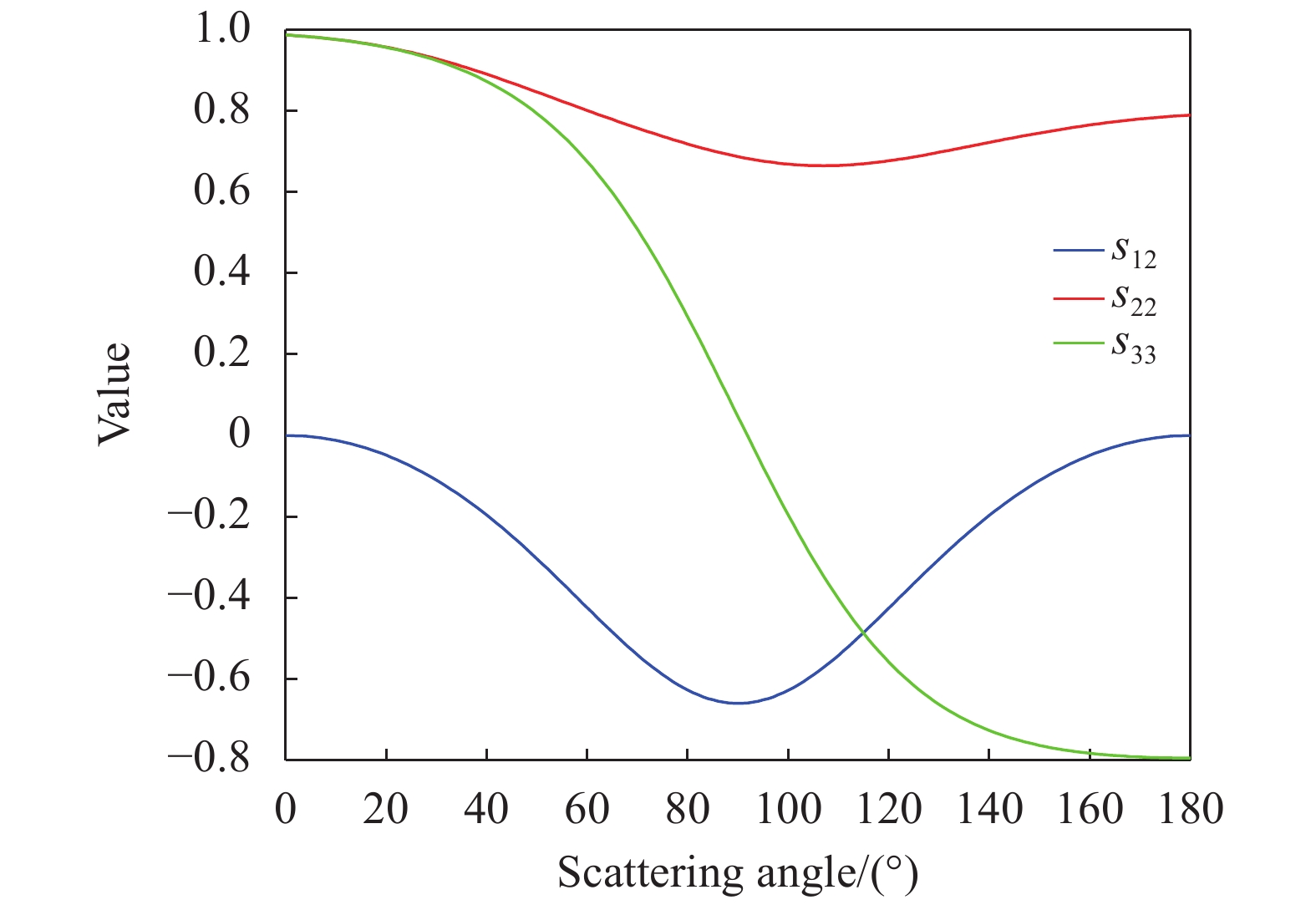
$$\begin{array}{l} {s_{12}}(\theta ) = - \dfrac{{s(90^\circ ){{\sin }^2}\theta }}{{1 + s(90^\circ ){{\cos }^2}\theta }} \\ {s_{22}}(\theta ) = \dfrac{{s(90^\circ )(1 + {{\cos }^2}(\theta - {\theta _0})) + \xi \exp ( - \mu \theta )}}{{1 + s(90^\circ ){{\cos }^2}(\theta - {\theta _0}) + \xi \exp ( - \mu \theta )}} \\ {s_{33}}(\theta ) = \dfrac{{2s(90^\circ )\cos \theta + \xi \exp ( - \mu \theta )}}{{1 + s(90^\circ ){{\cos }^2}\theta + \xi \exp ( - \mu \theta )}} \\ \end{array} $$ (4) 其中,偏振度s(θ)≡−s12(θ),粒子散射中s12、s22、s33与散射角的关系如图1所示。在公式(4)中,非偏振光(散射角为90°)的偏振度s(90°) = 0.66;引入θ0来描述s22(θ)取最小值时的散射角与90°之间的偏移,此处θ0为0.25 rad;用带有自由参数μ和ξ的指数函数ξexp(−μθ)来近似计算水中粒子在小角度发生多次散射时的s22(θ)和s33(θ),其中μ与θ0互为相反数,μ为4 rad−1,ξ为25.6。
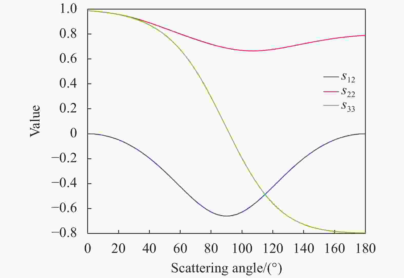
图 1 粒子散射中s12、s22、s33与散射角的关系
Figure 1. Relationship between s12, s22, s33 and particle scattering angle
-
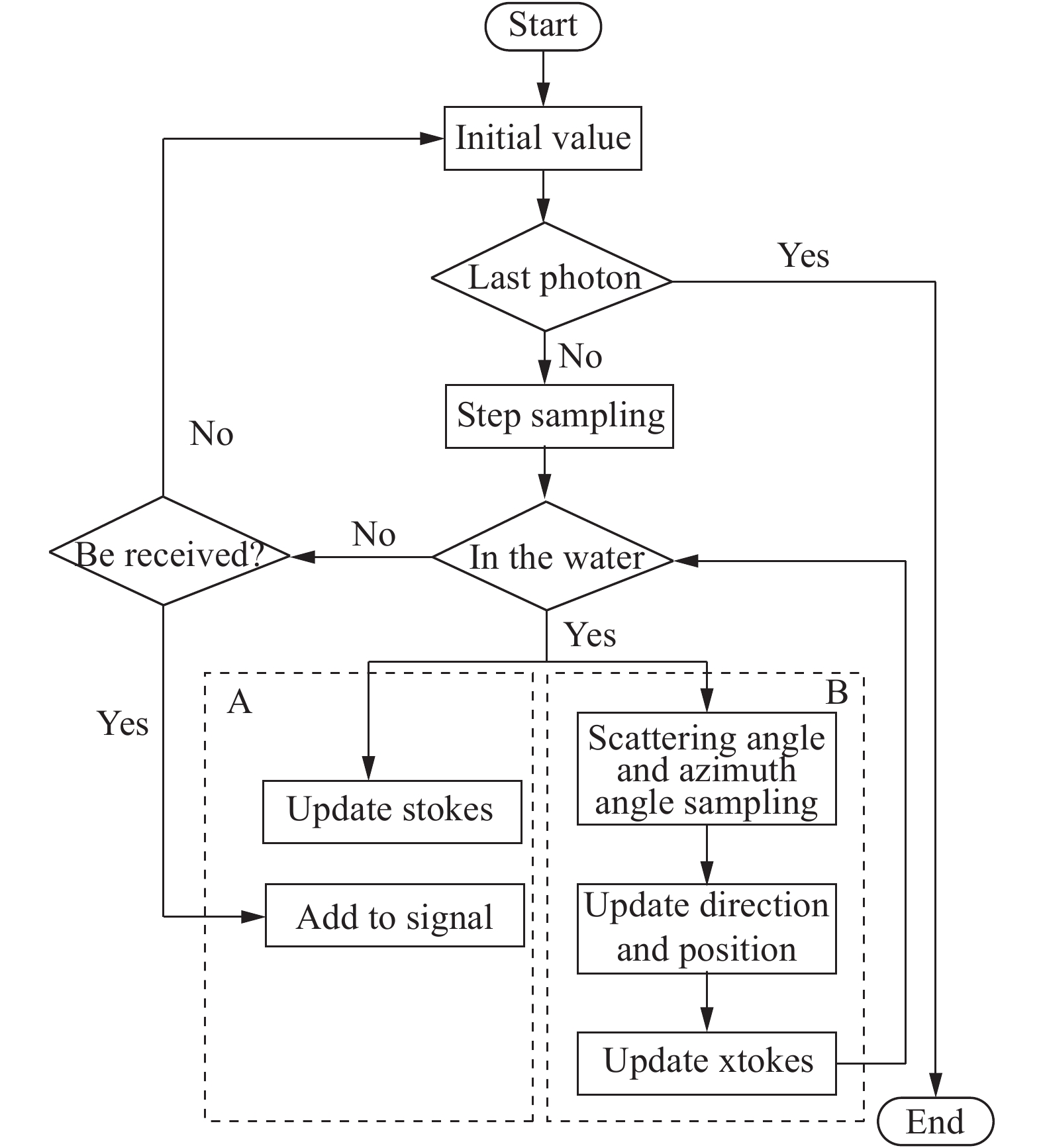
文中通过建立偏振蒙特卡洛子午面法传输模型对激光在海水中的辐射传输进行模拟仿真,并运用半分析法和统计权重法获得每个光子到达探测器的信号量从而加快模拟过程,偏振蒙特卡洛子午面法的仿真流程图如图2所示,图中A表示光子直接累加到探测器中心的部分,B表示光子在水下继续运动的部分。

图 2 偏振蒙特卡洛仿真流程图
Figure 2. Flowchart of polarization Monte Carlo simulation
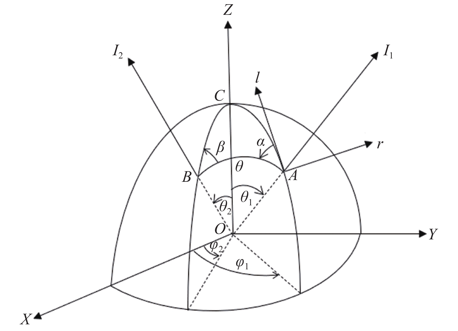
在偏振蒙特卡洛子午面仿真方法中,光的偏振状态是相对于参考面定义的,所以偏振蒙特卡洛仿真方法的一个重要特性是追踪用来描述光的偏振状态的三个参考面,分别是散射前的子午面、散射面和散射后的子午面,子午面和散射面的几何关系图如图3所示。

图 3 子午面和散射面的几何关系图
Figure 3. Geometric diagram of the meridian and scattering planes
将垂直于海面向下的方向设置为三维坐标轴中Z轴的正方向,光子沿Z轴正方向入射,初始方向余弦(ux,uy,uz)=(0,0,1),初始位置坐标(x0,y0,z0)=(0,0,0),初始光子权重w = 1,初始偏振状态S0=[1 1 0 0]T,初始子午面是XOZ平面。
光子散射一次后的几何运动路径长度为:
$r = - \dfrac{1}{c}\ln (\xi )$ ,ξ是0~1之间均匀分布的随机数,c(m−1)是海水衰减系数。在偏振蒙特卡洛算法中,光子在每一次碰撞之后的散射方向均由图3中的散射角θ和旋转角α决定,因此偏振蒙特卡洛算法中的一个基本问题是基于散射相函数,利用“拒绝法”[12]对散射角θ和旋转角α进行选择,散射相函数的表示如下:
$$P(\theta ,\alpha ) = {M_{11}}(\theta ){I_0} + {M_{12}}(\theta )({Q_0}\cos 2\alpha + {U_0}\sin 2\alpha )$$ (5) 式中:S0 =[I0 Q0 U0 V0]T表示入射斯托克斯矢量;M11和M12是穆勒矩阵中的元素;M11是关于散射角θ的散射相函数;M12为散射相函数M11与散射相矩阵s中s12的乘积。采用“拒绝法”抽样产生三个随机变量Prand、θrand和αrand。其中,Prand是0~1之间均匀产生的随机偏差,θrand在0~π之间均匀分布,αrand在0~2π之间均匀分布;如果Prand ≤P(θrand, αrand),则表示θrand和αrand可以被选取,否则继续生成三个随机变量,直到θrand和αrand满足可以被选取的条件,结束抽样过程。当散射角θ和旋转角α确定后,根据球面余弦定律[13]计算光子散射后的天顶角θ2和方位角φ2。
$$\cos {\theta _2} = \cos {\theta _1}\cos \theta + \sin {\theta _1}\sin \theta \cos \alpha $$ (6) $${\varphi _2} = \left\{ \begin{array}{l} {\varphi _1} - \arccos \left( {\dfrac{{\cos \theta - \cos {\theta _1}\cos {\theta _2}}}{{\sin {\theta _1}\sin {\theta _2}}}} \right),(0 < \alpha < \pi ) \\ {\varphi _1} - \arccos \left( {\dfrac{{\cos \theta - \cos {\theta _1}\cos {\theta _2}}}{{\sin {\theta _1}\sin {\theta _2}}}} \right),(\pi < \alpha < 2\pi ) \\ \end{array} \right.$$ (7) 式中:θ1和φ1表示入射光的天顶角和方位角,初始值均为0。
已知光子入射方向余弦(ux,uy,uz),散射角θ和方位角φ求解后,根据坐标旋转公式得到光子出射方向余弦(ux',uy',uz'):
$$\left[ {\begin{array}{*{20}{c}} {u_x'} \\ {u_y'} \\ {u_z'} \end{array}} \right] = \left\{ \begin{array}{l} \left[ {\begin{array}{*{20}{c}} {{{{u_x}{u_{\textit{z}}}} / {\sqrt {1 - {u_{\textit{z}}}^2} }}}&{{{ - {u_y}} / {\sqrt {1 - {u_{\textit{z}}}^2} }}}&{{u_x}} \\ {{{{u_y}{u_{\textit{z}}}} / {\sqrt {1 - {u_{\textit{z}}}^2} }}}&{{{{u_x}} / {\sqrt {1 - {u_{\textit{z}}}^2} }}}&{{u_y}} \\ { - \sqrt {1 - {u_{\textit{z}}}^2} }&0&{{u_{\textit{z}}}} \end{array}} \right]\left[ {\begin{array}{*{20}{c}} {\sin \theta \cos \phi } \\ {\sin \theta \sin \phi } \\ {\cos \theta } \end{array}} \right],{u_{\textit{z}}}^2 < 1 \\ \left[ {\begin{array}{*{20}{c}} {\sin \theta \cos \phi } \\ {\sin \theta \sin \phi } \\ {sign({u_{\textit{z}}})\cos \theta } \end{array}} \right],{u_{\textit{z}}}^2 \approx 1 \\ \end{array} \right.$$ (8) 根据光子出射方向余弦和光子运动的几何路径长度,就可以计算光子下一次发生散射的位置:
$$\begin{split} {x'} = x + {u_x}'r \\ {y'} = y + {u_y}'r \\ {{\textit{z}}'} = {\textit{z}} + {u_z}'r \\ \end{split} $$ (9) 初始入射光的斯托克斯矢量是根据子午线平面COA来定义的,光子在水下继续运动的部分用“拒绝法”生成散射角θ和旋转角α后,需要对斯托克斯矢量进行三次旋转操作。首先斯托克斯矢量与旋转矩阵R(−α)相乘,参考平面从子午面COA逆时针旋转α到散射面AOB;接着旋转后的斯托克斯矢量与穆勒矩阵M(θ)相乘得到散射后的斯托克斯矢量;最后散射后的斯托克斯矢量与旋转矩阵R(π−β)相乘,参考平面从散射面AOB逆时针旋转β到子午面COB。散射面AOB与散射后子午面COB之间的旋转角β通过球面余弦定律得到:
$$\beta = \left\{ \begin{array}{l} \arccos \left( {\dfrac{{\cos {\theta _1} - \cos {\theta _2}\cos \theta }}{{\sin {\theta _2}\sin \theta }}} \right),(0 < \alpha < \pi ) \\ 2\pi - \arccos \left( {\dfrac{{\cos {\theta _1} - \cos {\theta _2}\cos \theta }}{{\sin {\theta _2}\sin \theta }}} \right),(\pi < \alpha < 2\pi ) \\ \end{array} \right.$$ (10) 假设光子在水中发生散射前的斯托克斯矢量为[I Q U V]T,则光子在水中继续散射后的斯托克斯矢量[Is Qs Us Vs] T可表示为:
$$\left[ {\begin{array}{*{20}{c}} {{I_s}} \\ {{Q_s}} \\ {{U_s}} \\ {{V_s}} \end{array}} \right] = R(\pi - \beta )M(\theta )R( - \alpha )\left[ {\begin{array}{*{20}{c}} I \\ Q \\ U \\ V \end{array}} \right]$$ (11) 在直接散射到探测器中心的部分中,需要构想光子从海面以下到达探测器中心的运动路径,即光子在海水中朝某方向运动,经过海面折射后恰好到达探测器中心。假设光子在水中发生散射前的斯托克斯矢量为[I Q U V]T,根据Hu等人在2001年运用的期望值方法[14]计算到达探测器的光子的斯托克斯矢量[Id Qd Ud Vd] T:
$$\left[ {\begin{array}{*{20}{c}} {{I_d}} \\ {{Q_d}} \\ {{U_d}} \\ {{V_d}} \end{array}} \right] = {\omega _0}\Delta \Omega {e^{ - cd}}{T_{atm}}{T_{sur}}R( - \gamma )R(\pi - \beta )M(\theta )R( - \alpha )\left[ {\begin{array}{*{20}{c}} I \\ Q \\ U \\ V \end{array}} \right]$$ (12) 式中:ΔΩ表示接收立体角,此处表示光子在接收立体角内散射的概率;c是海水衰减系数;d是光子在海面发生折射的位置光子与水中散射点之间的距离;e−cd即表示光子从海水到达海面过程中不与海水中任何分子或颗粒物发生碰撞的概率;Tatm表示大气透过率;Tsur表示海气界面透过率;ω0是单次反照率;θ是散射角;α是散射前子午面与散射面之间的夹角;β是散射面与散射后子午面之间的夹角;γ是光子到达探测器中心时的运动方向跟Z轴形成的子午面与探测器子午面XOZ之间的夹角。α和β的求解过程如下:
$$\begin{array}{l} \cos \alpha = \dfrac{{\cos {\theta _{sca}} - \cos {\theta _{inc}}\cos \theta }}{{\sin {\theta _{inc}}\sin \theta }} \\ \cos \beta = \dfrac{{\cos {\theta _{inc}} - \cos {\theta _{sca}}\cos \theta }}{{\sin {\theta _{sca}}\sin \theta }} \\ \end{array} $$ (13) 当sin θ = 0时,cos α = 1,cos β = 1;当sin θinc = 0时:
$$\begin{array}{l} \cos \alpha = - \cos {\theta _{inc}}\cos ({\phi _{sca}} - {\phi _{inc}}) \\ \cos \beta = \cos {\theta _{inc}} \\ \end{array} $$ (14) 当sin θsca = 0时,
$$\begin{array}{l} \cos \alpha = - \cos {\theta _{sca}}\cos ({\phi _{sca}} - {\phi _{inc}}) \\ \cos \beta = \cos {\theta _{sca}} \\ \end{array} $$ (15) 式中:θ为散射角;θinc表示入射光的天顶角,即入射光与Z轴正方向的夹角;φinc为入射光的方位角;θsca表示散射光的天顶角;φsca为散射光的方位角。
退偏振比δ由最终到达探测器的后向散射信号[Id Qd Ud Vd] T得到:
$$\delta = ({I_d} - {Q_d})/({I_d} + {Q_d})$$ (16) 对于激光与海水中分子或粒子发生单次散射后产生的回波信号,单次散射退偏振比δs表示为:
$$ \begin{split} {\delta _s} =& \dfrac{{{M_{11}}(180^\circ ) - {M_{22}}(180^\circ )}}{{{M_{11}}(180^\circ ) + {M_{22}}(180^\circ )}} \dfrac{{{s_{11}}(180^\circ ) - {s_{22}}(180^\circ )}}{{{s_{11}}(180^\circ ) + {s_{22}}(180^\circ )}} =\\ & \dfrac{{1 - {s_{22}}(180^\circ )}}{{1 + {s_{22}}(180^\circ )}} \\ \end{split} $$ (17) 光在海洋水体中发生粒子散射时s(90°)为0.66[11],由此可以计算单次散射退偏振比δs为0.1173。
-
文中采用自然海洋水域中粒子散射的散射相矩阵,利用偏振蒙特卡洛仿真模型模拟垂直剖面水体中,船载海洋激光雷达垂直偏振通道和平行偏振通道的回波信号,仿真参数如表1所示。
表 1 船载海洋激光雷达仿真参数
Table 1. Parameters for simulation of shipborne oceanographic lidar
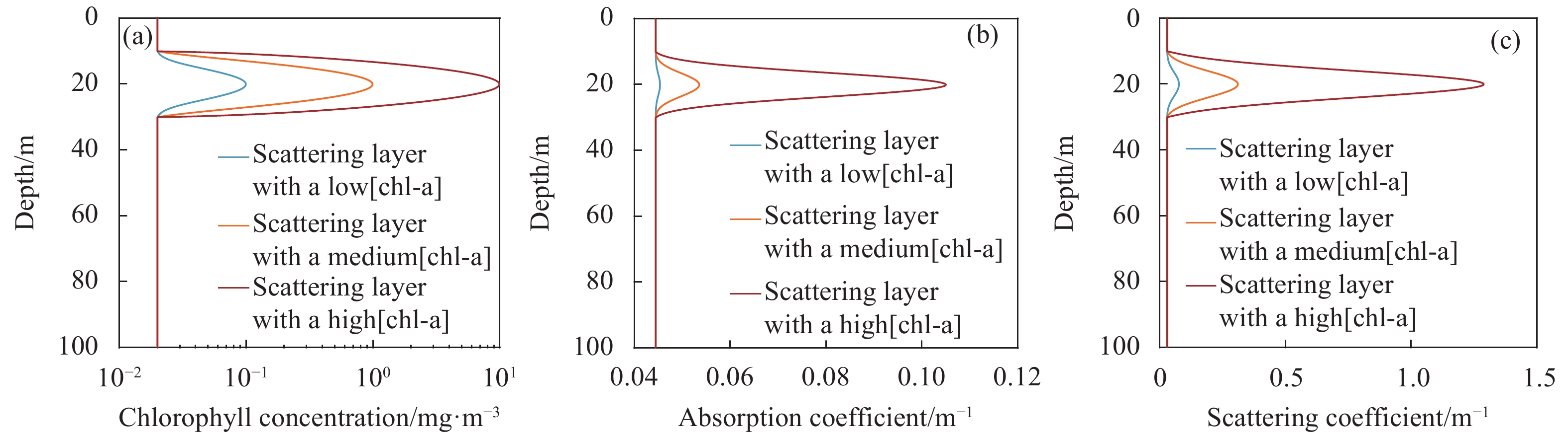
Parameters Value Laser wavelength/nm 532 Telescope diameter/m 0.3 Field of view/mrad 10, 20, 50, 100, 200, 500, 1000 Platform height/m 5 Phase function Petzold Transmission photon counts 107 Maximum scattering times 20 Profile resolution/m 0.1 文中使用高斯分布设置了三种深度分布在10~30 m的低、中、高浓度散射层,在深度20 m处出现叶绿素a浓度峰值,分别为0.1 mg/m3、1 mg/m3和10 mg/m3,背景叶绿素a浓度均为0.02 mg/m3,低、中、高浓度散射层情况下的叶绿素a浓度剖面如图4(a)所示。水体总吸收系数为纯水吸收系数与叶绿素a吸收系数之和,纯水的吸收系数采用Pope和Fry[15]的测量结果,叶绿素a的吸收系数使用Lee[16]等人建立的浮游植物吸收光谱的参数化表达式计算得到。水体总散射系数为纯水散射系数与叶绿素a散射系数之和,纯水散射系数采用Morel[17]模型,叶绿素a散射系数采用Gordon和Morel[18]提出的关于浮游植物散射系数的计算公式。水体总吸收系数剖面和总散射系数剖面分别如图4(b)和4(c)所示。
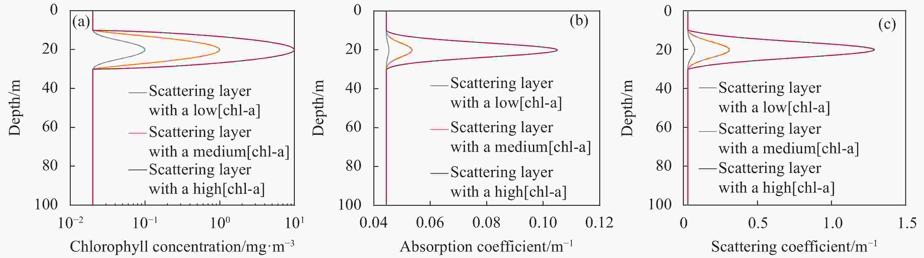
图 4 (a)低、中、高散射层水体的叶绿素a浓度剖面;(b)水体总吸收系数a剖面;(c)水体总散射系数b剖面
Figure 4. (a) Profile of chlorophyll-a concentration in low, medium and high scattering layer; (b) Absorption coefficient a profile; (c) Scattering coefficient b profile
深度剖面分辨率为1 m的船载海洋激光雷达仿真回波信号如图5所示,图中(a)、(b)、(c)分别对应低、中、高浓度散射层的情况,实线表示平行通道的回波能量,虚线表示垂直通道的回波能量。将0~40 m深度分为散射层上(0~10 m)、散射层中(10~30 m)和散射层下(30~40 m)三个深度区间。
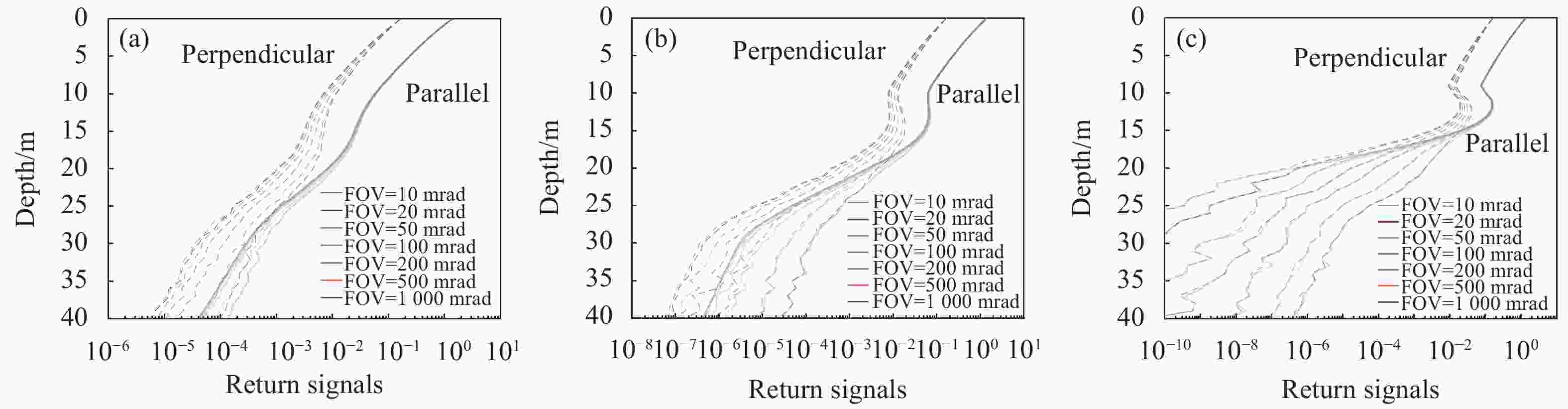
图 5 (a)低、(b)中、(c)高散射层水体中的船载海洋激光雷达仿真回波信号
Figure 5. Simulated shipborne oceanographic lidar return signals in (a) low, (b) medium and (c) high scattering layer
在散射层上(0~10 m),水体吸收系数和散射系数随深度不改变,可以看作均匀水体,回波曲线变化较为平缓。这一部分中回波能量随深度缓慢衰减,平行偏振通道在不同视场角下的衰减基本不变,三种情况的垂直通道回波曲线变化几乎一致,视场越大衰减越慢。
在散射层中(10~30 m)水体的吸收系数和散射都随颗粒物浓度增大,对光信号的衰减和散射作用都更强,二者共同作用下,随着深度的增加,散射层内的回波信号在的衰减趋势会先变缓(低浓度散射层情况)甚至增强(中浓度、高浓度散射层情况),随后以更快的速度衰减。其中高浓度散射层的衰减程度最严重,中浓度散射层的次之,低浓度散射层的衰减程度最低。另外,在散射层中,颗粒物浓度的增加会导致多次散射增多,这时在深度较大处的光子大部分是多次散射之后到达的,因此水平偏振通道的回波信号较垂直偏振通道衰减更快,在大视场角情况下更为明显,中、高浓度散射层情况下两通道的回波能量在某一深度处开始出现重合。高浓度散射层情况下,在深度25 m以下,回波信号已经完全退偏,因此两通道的信号基本重合。
船载海洋激光雷达仿真回波信号的退偏振比(根据公式(16)计算得到)剖面如图6所示,图中(a)、(b)、(c)分别对应低、中、高浓度散射层的情况。三种水体在海面处的退偏振比均约为0.118,略大于单次散射退偏振比0.1173,退偏振比随深度、叶绿素a浓度和视场角的增加逐渐变大。在散射层以上,由于水体参数相同,低、中、高三种浓度散射层情况的退偏振比随深度和视场角的变化趋势相同。
在散射层中和散射层下,不同水体不同视场角的退偏振比均随深度增大。低、中浓度散射层情况在小视场角下的退偏振比随深度变化较小,而高浓度散射层情况的退偏振比无论视场角大小,均在散射层出现一段时间后产生很大变化,深度为25 m左右时高浓度散射层情况在各个视场角下的退偏振比趋于饱和。
由于假定的水体颗粒物退偏振系数为常数,因此退偏振比相对误差随深度、散射层浓度和视场角的变化规律与退偏振比的变化趋势一致。

图 6 (a)低、(b)中、(c)高散射层水体中的船载海洋激光雷达回波信号的退偏振比剖面
Figure 6. Depolarization ratio profiles from shipborne oceanographic lidar return signals in (a) low, (b) medium and (c) high scattering layer
-
海洋激光雷达回波信号的退偏振程度不仅受到水体颗粒物退偏振比的影响,而且还取决于多次散射作用的程度。
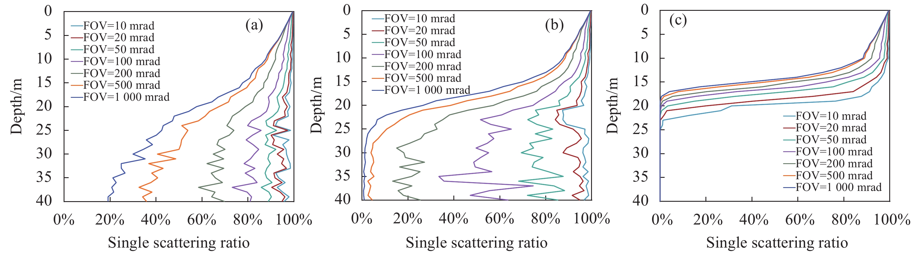
激光雷达接收到的单次散射信号在总接收信号中的占比(简称单次散射率)能够反映发生多次散射的情况,单次散射率越低的地方,发生的单次散射越少,多次散射越多。船载海洋激光雷达仿真回波信号的单次散射率剖面如图7所示,图中(a)、(b)、(c)分别对应低、中、高浓度散射层水体的情况。

图 7 (a)低、(b)中、(c)高散射层水体中的船载海洋激光雷达仿真回波信号的单次散射率剖面
Figure 7. Single scattering ratio profiles of simulated shipborne oceanographic lidar return signals in (a) low, (b) medium and (c) high scattering layer
深度越大,回波信号受到多次散射的影响越大,单次散射率越低;叶绿素a浓度越大,粒子分布越密集,光子与某一粒子发生碰撞后再与周围其他粒子发生碰撞的概率就会越大,多次散射会越多;视场角越大,接收器接收到的多次散射信号也会越多。因此,多次散射会随会随探测深度、叶绿素a浓度和接收视场角的增大不断增多,单次散射率就会不断减小。
文中假定的水体颗粒物的实际退偏振比为一个常值(0.1173,由公式(17))。由于激光在水中的多次散射过程,随着探测深度、叶绿素a浓度和接收视场角的增大,激光雷达接收光信号的单次散射率不断降低,导致激光雷达回波信号退偏振程度增大,直接测量的退偏振比的误差随之增大。
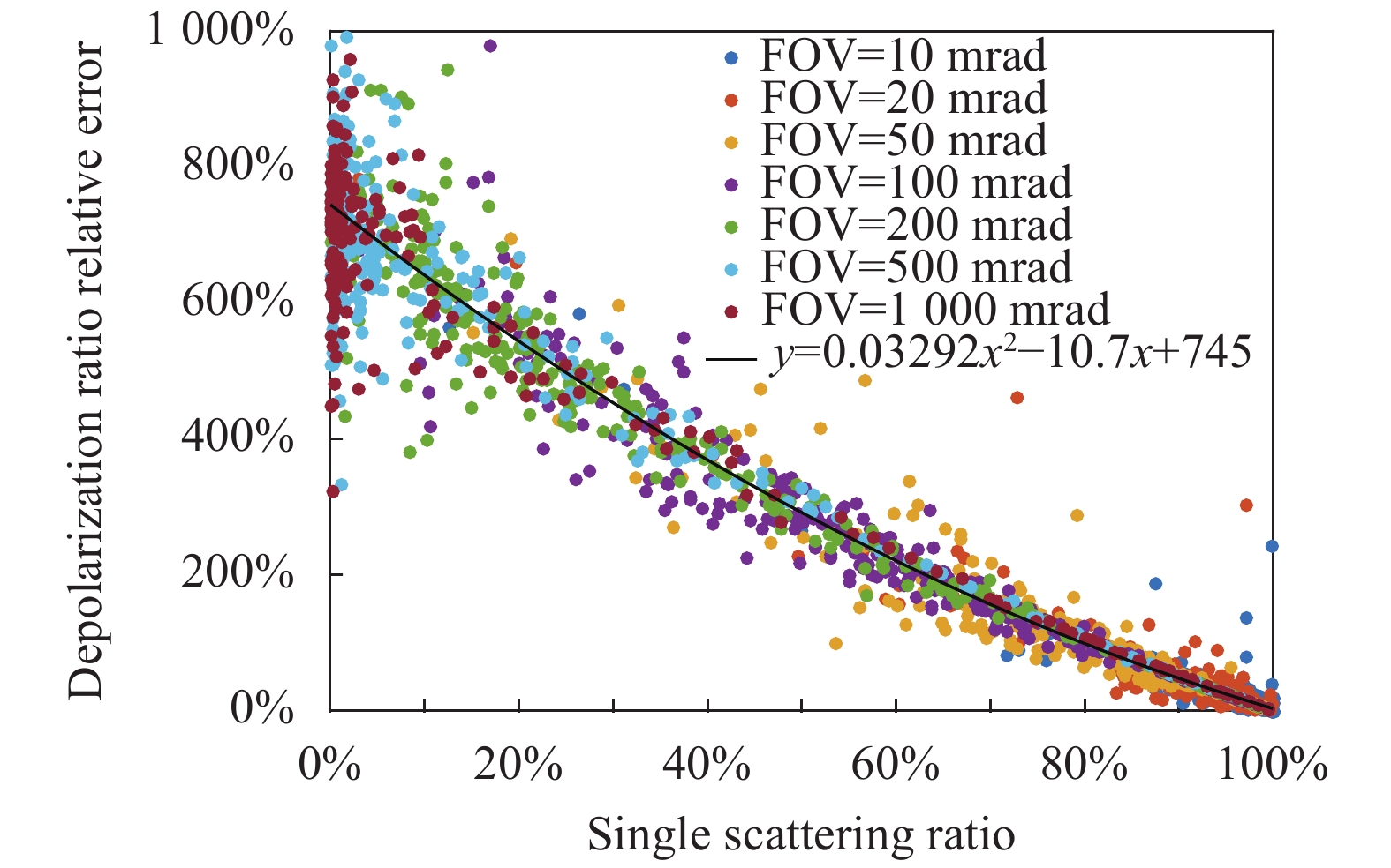
单次散射率与退偏振比相对误差的关系如图8所示。图中散点包含了低、中、高三种散射层浓度的情况,不同视场角用不同的颜色表示,黑色实线表示所有散点的二次多项式拟合。图中单次散射率与退偏振比相对误差呈负相关,退偏振比测量误差随单次散射率的减小而增大。在不同深度、颗粒物浓度和视场角情况下,退偏振比测量误差和单次散射率的关系呈现出一致的趋势,验证了单次散射率的降低是导致退偏振比误差增大的本质原因。

图 8 退偏振比相对误差与单次散射率的关系
Figure 8. Relationship between relative errors of depolarization ratio and single scattering ratios
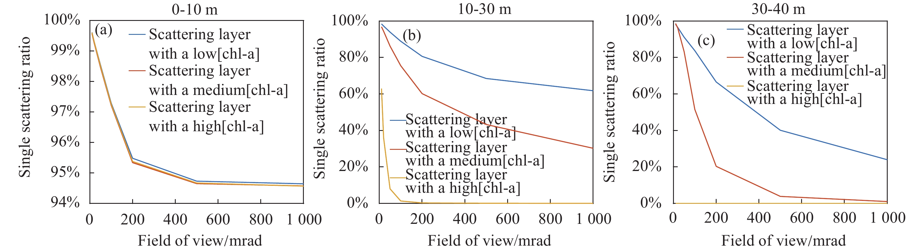
不同视场角情况下的单次散射率和退偏振比相对误差分别如图9和图10所示,两图中(a)、(b)、(c)分别对应散射层上、散射层中、散射层下的部分。随视场角的增大,由于

图 9 散射层(a)以上、(b)之中、(c)以下深度处的单次散射率与视场角的关系
Figure 9. Relationship between single scattering ratio and field of view (a) above, (b) in and (c) below the scattering layer
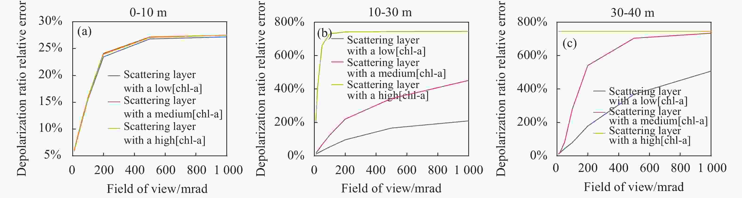
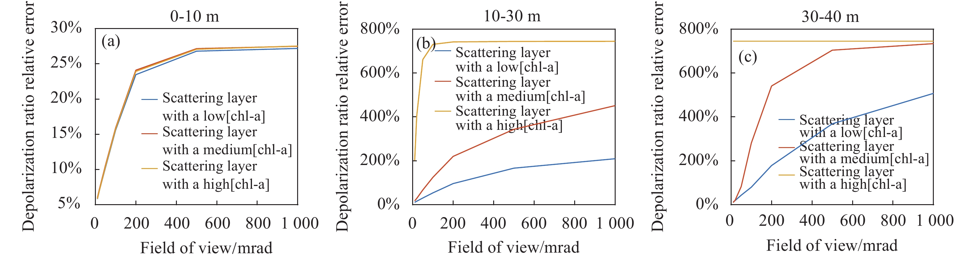
图 10 散射层(a)以上、(b)之中、(c)以下深度处的退偏振比相对误差与视场角的关系
Figure 10. Relationship between relative errors of depolarization ratio and field of view (a) above, (b) in and (c) below the scattering layer
激光雷达接收到的多次散射信号增多,其单次散射率整体上呈减小趋势(如图9所示),正是由于单次散射率的减小,激光雷达直接探测的退偏振比误差整体上呈增大趋势(如图10所示)。以中浓度散射层情况为例,视场角从10 mrad增大到1000 mrad时,单次散射率在散射层上从99%减少至95%,在散射层中从97%减少至30%,在散射层下从99%减少至1%。受其影响,退偏振比测量误差在散射层上从6%增加28%,在散射层中从17%增加452%,在散射层下从10%增加734%。同种浓度散射层水体情况下,视场角越大,由于接收到的多次散射信号越多,单次散射率越低,退偏振比测量误差越大。不同浓度散射层中,在散射层上的单次散射率和退偏振比测量误差在不同视场角下的数值均接近,散射层中与散射层下,受到散射层颗粒物浓度的影响,单次散射率和退偏振比测量误差的数值差异较大。
另外,在相同视场角情况下,由于颗粒物散射强度会改变多次散射的强度,从而影响激光雷达信号的单次散射率和退偏振比测量误差。以100 mrad视场角为例,在散射层上,由于不同浓度散射层情况的多次散射特征相同,其单次散射率和退偏振比变化趋势基本一致,低、中、高三种浓度散射层情况的单次散射率均为97% (图9(a)),退偏振比相对误差均为16%(图10(a));在散射层中,低、中、高三种浓度散射层中的多次散射依此增加,单次散射率分别为89%、76%、1% (图9(b)),退偏振比误差分别为54%、125%、731% (图10(b));在散射层以下,多次散射信号仍然受到散射层的影响,单次散射率分别为84%、52%、0% (图9(c)),退偏振比误差分别为80%、281%、745% (图10(c))。
-
文中利用偏振蒙特卡洛子午面法建立了水中激光偏振辐射传输模型,在低、中、高浓度散射层水体情况下,分别仿真模拟了船载偏振海洋激光雷达在不同接收视场角(10~1000 mrad)时的垂直偏振通道和平行偏振通道的回波信号,分析了不同光学参数的水体和激光雷达测量模式下的水体垂直剖面的偏振测量误差及影响偏振测量误差的主要因素。
研究结果表明,由于激光在水中的多次散射过程,随着探测深度、叶绿素a浓度和接收视场角的增大,激光雷达接收光信号的单次散射率不断降低,导致激光雷达直接测量的退偏振比的误差随之增大。
(1)随深度变化:视场角为100 mrad时,中浓度散射层情况在散射层上、散射层中和散射层下的单次散射率分别为97%、76%、52%,退偏振比相对误差分别为16%、125%、281%。
(2)随散射层浓度变化:同一视场角下低浓度散射层情况的单次散射率最高,退偏振比测量误差最小,中浓度和高浓度散射层的单次散射率和退偏振比误差依次变化。低、中、高三种浓度散射层在散射层中的退偏振比相对误差约为54%、125%、731%。
(3)随视场角的变化:视场角越大,退偏振比测量误差越大,中叶绿素a浓度散射层情况下,视场角从10 mrad增大到1000 mrad时,退偏振比相对误差在散射层上从6%增加28%,在散射层中从17%增加452%,在散射层下从10%增加734%。
文中结果表明,多次散射是偏振海洋激光雷达水体退偏振比测量误差增大的本质原因。作为描述多次散射程度的定量参数,单次散射率是退偏振比误差重要决定因素。传统的基于单次散射假设的退偏振比算法会引入较大误差,有必要在反演算法中对其进行校正,以提高激光雷达的探测精度。
Simulation of polarization profiles of water measured by oceanographic lidar
-
摘要:
基于蒙特卡洛模拟方法,建立了一个水中激光偏振辐射传输模型,用于模拟分析船载偏振激光雷达水体垂直剖面的偏振探测回波,分析了不同光学参数的水体和激光雷达测量模式下的偏振测量误差。使用高斯分布设置了三种深度分布在10~30 m的低、中、高浓度散射层,其叶绿素a峰值浓度分别为0.1 mg/m3、1 mg/m3和10 mg/m3。模拟了激光发射波长为532 nm,接收视场角为10~1000 mrad的船载海洋激光雷达的偏振回波信号,并分析了影响偏振测量误差的主要因素。研究结果表明,由于激光在水中的多次散射过程,随着探测深度、叶绿素a浓度和接收视场角的增大,激光雷达接收光信号的单次散射率不断降低,导致激光雷达直接测量的退偏振比的误差随之增大。以100 mrad接收视场角为例,中浓度散射层情况下,在散射层上(0~10 m)、散射层中(10~30 m)和散射层下(30~40 m)的退偏振比相对误差分别为16%、125%、281%;在散射层中,低、中、高三种浓度散射层的退偏振比相对误差分别为54%、125%、731%。视场角从10 mrad增大到1000 mrad时,退偏振比相对误差逐渐增大,在中浓度散射层情况下,其在散射层上、散射层中和散射层下的变化范围分别为6%~28%、17%~452%和10%~734%。文中结果表明,偏振海洋激光雷达探测水体退偏振比时,由于多次散射过程的影响,传统的退偏振比算法会引入较大误差,有必要在反演算法中对其进行校正,以提高激光雷达的探测精度。
Abstract:A Monte Carlo radiative transfer model with polarization was developed to simulate and analyze the vertical profile of received polarization signal of a ship-borne lidar. The measurement errors resulted from different seawater optical parameters and various lidar measurement modes were analyzed as well. A Gaussian distribution function was used to describe the chlorophyll-a vertical profile. The scattering layers were set at 10-30 m with the low, medium and high values of chlorophyll-a concentration ([chl-a]), respectively, and the corresponding maximum value of [chl-a] was 0.1 mg/m3, 1 mg/m3 and 10 mg/m3, respectively. The polarization return signals of the ship-borne oceanographic lidar were simulated with a laser transmission wavelength of 532 nm and field of views (FOVs) of 10-1000 mrad, and the main factors affecting the polarization measurement error were analyzed. The results suggest that the single scattering ratio of lidar return signal decreases with the enhancements of detection depth, [chl-a] and FOV due to the multiple scattering process of laser transferring in seawater. This leads to an increase in the error of the depolarization ratio directly measured by lidar. Let’s take the FOV of 100 mrad as an example. In the case of the scattering layer with a medium [chl-a], the relative errors of the depolarization ratio above (0-10 m), in (10-30 m) and under (30-40 m) the scattering layer were 16%, 125% and 281%, respectively. In the scattering layer, the relative errors of the depolarization ratio were 54%, 125% and 731% for the low, medium and high values of [chl-a], respectively. When the FOV increases from 10 mrad to 1000 mrad, the relative error of the depolarization ratio increases from 6%-28% above the scattering layer, 17%-452% in the scattering layer and 10%-734% under the scattering layer, respectively, for the case of the scattering layer with a medium [chl-a]. Therefore, when using the polarization oceanographic lidar to detect the seawater depolarization ratio, the traditional algorithm for depolarization ratio will introduce a large error due to the multiple scattering process, and a correction is required to improve the detection accuracy of lidar measurement.
-
图 1 粒子散射中s12、s22、s33与散射角的关系
Figure 1. Relationship between s12, s22, s33 and particle scattering angle
图 4 (a)低、中、高散射层水体的叶绿素a浓度剖面;(b)水体总吸收系数a剖面;(c)水体总散射系数b剖面
Figure 4. (a) Profile of chlorophyll-a concentration in low, medium and high scattering layer; (b) Absorption coefficient a profile; (c) Scattering coefficient b profile
图 5 (a)低、(b)中、(c)高散射层水体中的船载海洋激光雷达仿真回波信号
Figure 5. Simulated shipborne oceanographic lidar return signals in (a) low, (b) medium and (c) high scattering layer
图 6 (a)低、(b)中、(c)高散射层水体中的船载海洋激光雷达回波信号的退偏振比剖面
Figure 6. Depolarization ratio profiles from shipborne oceanographic lidar return signals in (a) low, (b) medium and (c) high scattering layer
图 7 (a)低、(b)中、(c)高散射层水体中的船载海洋激光雷达仿真回波信号的单次散射率剖面
Figure 7. Single scattering ratio profiles of simulated shipborne oceanographic lidar return signals in (a) low, (b) medium and (c) high scattering layer
图 8 退偏振比相对误差与单次散射率的关系
Figure 8. Relationship between relative errors of depolarization ratio and single scattering ratios
图 9 散射层(a)以上、(b)之中、(c)以下深度处的单次散射率与视场角的关系
Figure 9. Relationship between single scattering ratio and field of view (a) above, (b) in and (c) below the scattering layer
图 10 散射层(a)以上、(b)之中、(c)以下深度处的退偏振比相对误差与视场角的关系
Figure 10. Relationship between relative errors of depolarization ratio and field of view (a) above, (b) in and (c) below the scattering layer
表 1 船载海洋激光雷达仿真参数
Table 1. Parameters for simulation of shipborne oceanographic lidar
Parameters Value Laser wavelength/nm 532 Telescope diameter/m 0.3 Field of view/mrad 10, 20, 50, 100, 200, 500, 1000 Platform height/m 5 Phase function Petzold Transmission photon counts 107 Maximum scattering times 20 Profile resolution/m 0.1  下载: 导出CSV
-
[1] Collister L, Zimmerman C, Hill J, et al. Polarized lidar and ocean particles: insights from a mesoscale coccolithophore bloom [J]. Applied Optics, 2020, 59(15): 4650-4662. doi: 10.1364/AO.389845 [2] Weitkamp C. Lidar: Range-Resolved Optical Remote Sensing of the Atmosphere[M]. New York: Springer, 2005. [3] Hu Yongxiang, Liu Zhaoyan, Winker D, et al. Simple relation between lidar multiple scattering and depolarization for water clouds [J]. Optics Letters, 2006, 31(12): 1809-1811. doi: 10.1364/OL.31.001809 [4] Sun Xianming, Wan Long, Wang Haihua. Sensitivity study on lidar detection of the depolarization ratio of water clouds [J]. Infrared and Laser Engineering, 2016, 45(9): 0906001. (in Chinese) doi: 10.3788/IRLA201645.0906001 [5] Kong Xiaojuan, Liu Bingyi, Yang Qian, et al. Simulation of water optical property measurement with shipborne lidar [J]. Infrared and Laser Engineering, 2020, 49(2): 0205010. (in Chinese) doi: 10.3788/IRLA202049.0205010 [6] 刘群. 星载海洋激光雷达多次散射信号模拟与探测机理研究[D]. 浙江: 浙江大学, 2020. Liu Qun. Research on simulation and detection mechanism of multiple scattering signal of spaceborne oceanic lidar[D]. Hangzhou: Zhejiang University, 2020. (in Chinese) [7] 王勇. 利用偏振光散射区分悬浮颗粒物与海洋微藻分类的研究[D]. 北京: 清华大学, 2018. Wang Yong. A study on classification of suspended particles and marine microalgae by polarized light scattering[D]. Beijing: Tsinghua University, 2018. (in Chinese) [8] De Boer F, Milner E. Review of polarization sensitive optical coherence tomography and Stokes vector determination [J]. Journal of Biomedical Optics, 2002, 7(3): 359-371. doi: 10.1117/1.1483879 [9] Kattawar G, Adams C. Stokes vector calculations of the submarine light field in an atmosphere- ocean with scattering according to a rayleigh phase matrix: Effect of interface refractive index on radiance and polarization [J]. Limnology and Oceanography, 1989, 34(8): 1453-1472. doi: 10.4319/lo.1989.34.8.1453 [10] Voss J, Fry S. Measurement of the Mueller matrix for ocean water [J]. Applied Optics, 1984, 23(23): 4427-4439. doi: 10.1364/AO.23.004427 [11] Kokhanovsky A A. Parameterization of the Mueller matrix of oceanic waters [J]. Journal of Geophysical Research(Oceans), 2003, 108(C6): 3175. doi: https://doi.org/10.1029/2001JC001222 [12] Ramella-Roman C, Prahl A, Jacques L. Three Monte Carlo programs of polarized light transport into scattering media: part I [J]. Optics Express, 2005, 13(12): 4420-4438. doi: 10.1364/OPEX.13.004420 [13] Hovenier W, Mee C. Fundamental relationships relevant to the transfer of polarized light in a scattering atmosphere [J]. Astronomy and Astrophysics, 1983, 128: 1-16. [14] Hu Yongxiang, David W, Yan Ping, et al. Identification of cloud phase from PICASSO-CENA lidar depolarization: a multiple scattering sensitivity study [J]. Journal of Quantitative Spectroscopy and Radiative Transfer, 2001, 70(4): 569-579. [15] Pope M, Fry S. Absorption spectrum (380-700 nm) of pure water. II. Integrating cavity measurements [J]. Applied Optics, 1997, 36(33): 8710-8723. doi: 10.1364/AO.36.008710 [16] Lee Zhongping. Visible-infrared remote sensing model and applications for ocean waters[D]. USA: University of South Florida, 1994. [17] Andre M, Louis P. Analysis of variations in ocean color [J]. Limnology and Oceanography, 1977, 22(4): 709-722. doi: 10.4319/lo.1977.22.4.0709 [18] Gordon H, Morel A. Remote Assessment of Ocean Color for Interpretation of Satellite Visible Imagery[M]. New York: Springer New York, 1983. -

 点击查看大图
计量
- 文章访问数: 540
- HTML全文浏览量: 188
- 被引次数: 0