


 下载:
下载:


-
作为一款新型影像学临床诊断设备,皮肤反射式共聚焦显振镜利用皮肤中血红蛋白、黑色素和角蛋白等不同组织成分的折射率差异进行成像,为皮肤组织的实时观测提供有效的技术手段,在恶性皮肤肿瘤早期诊断、治疗后随访等方面发挥了愈发重要的作用[1-2]。为进一步实现皮肤病检查时的便捷性,需要发展手持式皮肤共聚焦显振镜,由于受到系统体积和重量限制,系统中的核心部件扫描振镜要采用单镜面式MEMS振镜实现二维扫描成像,该扫描方式使得采集到的图像存在较为严重的二维畸变,扭曲了皮肤组织真实的结构形态,如不对这种图像畸变进行校正,将不利于医生观察皮损组织真实形态、边界轮廓、结构特征等信息,直接影响临床诊断结果[3-4]。因此,需要在分析产生图像畸变机理的基础之上,实现畸变校正,将真实图像信息准确呈现,为皮肤疾病诊断奠定基础。
目前,针对共聚焦图像畸变的机理分析均基于两振镜配合的扫描方式[5-6],如双检流计振镜、共振振镜-检流计振镜及双共振振镜,上述系统形成的主要图像扫描畸变为双曲线枕形畸变,只需校正一维(快轴)方向畸变,通过推导图像各像素实际位置、振镜实际偏转角以及控制电压三者关系,这种方式计算量大,实现难度较高,静态扫描控制方式一定程度上影响成像速度。而针对其他图像畸变的各类校正方法及算法主要有建立投影变换模型校正[7-10]、基于标定算法校正[11-12]以及人工智能算法校正等。基于投影变换模型校正方法主要适用于鱼眼相机,包括采用球面透视投影模型[13-14]、经纬度模型[15-16]、双经度模型[17]以及柱面模型[18-19]。球面透视投影的方法运算量庞大、必须获取一定数量的采样点才能得到较为准确的畸变校正参数,而且校正后的图像呈现严重拉伸,直接影像图像质量;经纬度以及双经度模型是以引入极点的方式来实现图像映射关系,但是在极点周围依然存在图像拉伸现象;柱面模型则是设置引导方向,将图像沿着柱面导向展开,这种方式有效避免了图像拉伸,但会损失中心画面。而基于标定算法的校正方式最先由Tsai[20]提出,首先需要求解初始化参数,然后经过非线性优化来实现系统标定参数,并确定畸变系数;张正友标定法[21]首先通过建立畸变数学模型,再利用多幅不同位姿的标定板图像完成畸变参数标定,该算法需要明确畸变种类。人工智能算法校正方法[22-24]主要包括机器视觉、深度学习、BP神经网络等,这些方法均需要较大的采样数据量,系统模型的准确构建直接影响校正结果。
文中分析了单镜面型MEMS振镜二维扫描畸变机理,通过记录原始光栅畸变图像,基于Hessian矩阵提取光栅中心线,二维方向分别拾取特征点并设置参考线,采用基于最小二乘法的7次多项式插值拟合方法进行二维方向像素畸变校正量标定,最终实现图像二维畸变校正,通过残差分析评估证明该方法有效可行,能够满足皮肤在体实时成像检测需求。
-
基于MEMS扫描振镜的共聚焦成像系统如图1所示,激光束经过PBS棱镜,反射至MEMS扫描振镜,其镜面在一定光学摆角内进行高速二维扫描,之后光束经扫描透镜和筒镜进行扩束,经过
${\lambda}$ /4波片调制偏振态,最后由物镜聚焦于待测样本面,样本反射光束由原路返回,分别经过物镜、${\lambda}$ /4波片、筒镜、扫描透镜、MEMS振镜后到达PBS棱镜,经针孔透镜聚焦于光纤端面,由探测器将光信号转换为电信号,最后上位机重建出图像。
图 1 基于MEMS扫描振镜的反射式共聚焦成像系统
Figure 1. Reflectance confocal microscope based on MEMS
-
MEMS振镜工作机理如图2所示,一束激光入射至MEMS振镜镜面中心,反射至投影面XOY,从而形成一个扫描光点。单镜面型MEMS振镜由上位机通过串口发送指令给下位机主控板,同时实现X、Y两维方向驱动控制,镜面在X方向为正弦波、Y方向为锯齿波运动模式,最终在投影面形成二维扫描图像。

图 2 MEMS振镜工作机理
Figure 2. Working mechanism of MEMS
-
首先,镜面绕快轴偏转运动,在系统投影面处建立xyz坐标系(与图2中xyz坐标系一致),设镜面由原始位置1绕快轴转动
$\alpha $ 到达位置2,则反射光偏转角为$2\alpha $ ,以镜面在位置2处的法线方向、垂直法线方向以及平行xyz坐标系中y轴方向建立x0y0z0坐标系,将入射光向量沿x0和z0方向分解,如图3(a)所示,则入射光在x0y0z0坐标系下的单位向量为$\left( {\rm{sin}}\alpha , $ $ 0,{\rm{cos}} \alpha \right)$ ,经镜面反射后的反射光也沿x0和z0方向分解,如图3(b)所示,则反射光在x0y0z0坐标系下的单位向量为$\left( {{\rm{sin}} \alpha ,0, -{\rm{ cos}} \alpha } \right)$ 。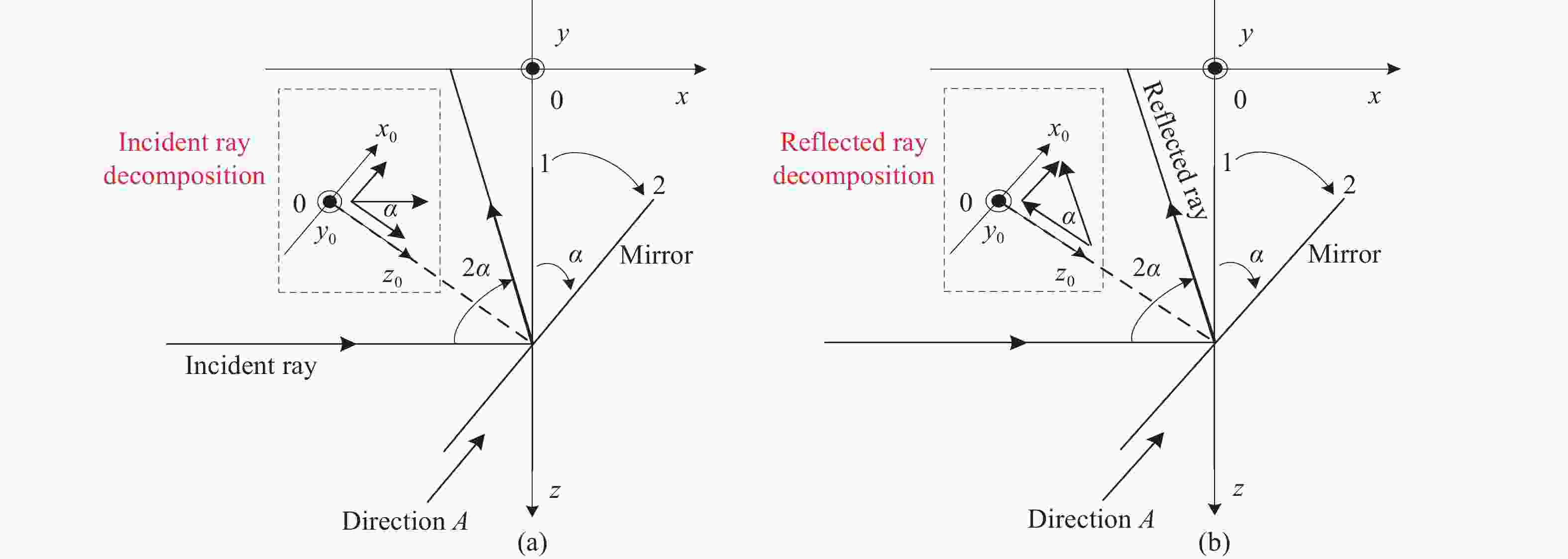
图 3 MEMS振镜绕快轴偏转运动示意图
Figure 3. Working around fast axis of MEMS
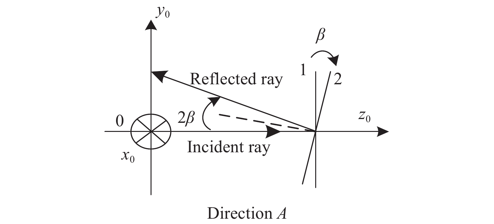
镜面绕慢轴偏转运动示意图如图4所示,其视图方向为图3中的A向,镜面由原始位置1绕慢轴转动
$\beta $ 到达位置2,则反射光偏转角为$2\beta $ 。反射光沿x0方向的分向量在振镜绕慢轴偏转运动过程中保持不变,因此其在x0方向上的单位向量仍为${{{\rm{sin}}}} \alpha $ ,将经过MEMS振镜二维偏转后的反射光在x0y0z0坐标系下分解,首先将反射光单位向量向y00z0平面投影,得出向量1的模为${\rm{sin}} \alpha $ ,向量2的模为${\rm{cos}} \alpha $ ,再将向量2向x00z0平面投影,得出向量3的模为${\rm{cos}} \alpha \cdot {\rm{sin}} 2\beta $ ,向量4的模为${\rm{cos}} \alpha \cdot {\rm{cos}} 2\beta $ ,考虑向量方向后得出反射光在x0y0z0坐标系下的单位向量可表示为$\left( {{{{\rm{sin}}}} \alpha ,{{{\rm{cos}}}} \alpha \cdot {{{\rm{sin}}}} 2\beta , - {{{\rm{cos}}}} \alpha \cdot {{{\rm{cos}}}} 2\beta } \right)$ 。
图 4 MEMS振镜绕慢轴偏转运动示意图
Figure 4. Working around slow axis of MEMS
在xyz坐标系下,将反射光在x0y0z0坐标系下的单位向量进行二次分解,则x0y0z0坐标系下x0方向的单位向量
${\rm{sin}} \alpha $ 在xyz坐标系下分解为$( {\rm{sin}}^2\alpha , 0, $ $ - {\rm{sin}}\alpha \cdot {\rm{cos}} \alpha)$ ,y0方向的单位向量${\rm{cos}} \alpha \cdot {\rm{sin}} 2\beta $ 分解为$\left( {0,{\rm{cos}} \alpha \cdot {\rm{sin}} 2\beta ,0} \right)$ ,z0方向的单位向量$ - {\rm{cos}} \alpha \cdot {\rm{cos}} 2\beta $ 分解为$\left( {{{{\rm{cos}} }^2}\alpha \cdot {\rm{cos}} 2\beta ,0, {\rm{sin}} \alpha \cdot {\rm{cos}} \alpha \cdot {\rm{cos}} 2\beta } \right)$ 。因此,将二次分解后的向量在xyz坐标系下重新沿各轴累加,可得出反射光在xyz坐标系下的单位向量如下:$\left( {{{{\rm{sin}} }^2}\alpha + {{{\rm{cos}} }^2}\alpha \cdot {\rm{cos}} 2\beta ,{\rm{cos}} \alpha \cdot {\rm{sin}} 2\beta , - {\rm{sin}} \alpha \cdot {\rm{cos}} \alpha + {\rm{sin}} \alpha \cdot {\rm{cos}} \alpha \cdot {\rm{cos}} 2\beta } \right)$ 反射光在xyz坐标系下的直线方程式可表示为:$$\left\{ {\begin{array}{*{20}{l}} {x = k \cdot \left( {{{{\rm{sin}} }^2}\alpha + {{{\rm{cos}} }^2}\alpha \cdot {\rm{cos}} 2\beta } \right)} \\ {y = k \cdot {\rm{cos}} \alpha \cdot {\rm{sin}} 2\beta } \\ {{\textit{z}} = L + k \cdot \left( { - {\rm{sin}} \alpha \cdot {\rm{cos}} \alpha + {\rm{sin}} \alpha \cdot {\rm{cos}} \alpha \cdot {\rm{cos}} 2\beta } \right)} \end{array}} \right.$$ (1) 式中:
$k$ 为系数;L为镜面至投影面XOY的距离。为了求解出投影面XOY上的二维图像,令公式(1)中${\textit{z}} = 0$ ,可得出:$$ {y^2} = \dfrac{{2L}}{{{\rm{tan}} \alpha }} \cdot x + \left( {\frac{1}{{{{{\rm{tan}} }^2}\alpha }} - 1} \right) \cdot {L^2} $$ (2) 由于实际情况下MEMS振镜镜面与入射光原始夹角为
$45^\circ $ ,因此,${\alpha _0} = 45^\circ $ ,${\;\beta _0} = 0^\circ $ ,绕快轴的机械偏转角约为$ \pm 7^\circ $ ,即$\alpha \in \left[ {38^\circ ,52^\circ } \right]$ ,绕慢轴的机械偏转角约为$ \pm 5^\circ $ ,即$\beta \in \left[ { - 5^\circ ,5^\circ } \right]$ 。令
$A\left( \alpha \right) = \dfrac{{2L}}{{{\rm{tan}} \alpha }}$ ,$B\left( \alpha \right) = \left( {\dfrac{1}{{{{{\rm{tan}} }^2}\alpha }} - 1} \right) \cdot {L^2}$ ,则公式(3)可化简为${y^2} = Ax + B$ ,图形为二次抛物线,由二次函数特性可知:当$A > 0$ 时,抛物线开口向右;当$A < 0$ 时,抛物线开口向左;$\left| A \right|$ 越大,抛物线开口越大;当$B > 0$ 时,抛物线与$x$ 轴交点在$y$ 轴左侧;当$B < 0$ 时,抛物线与$x$ 轴交点在$y$ 轴右侧;当$B = 0$ 时,抛物线与$x$ 轴交点为原点。函数
$A\left( \alpha \right) = \dfrac{{2L}}{{{\rm{tan}} \alpha }}$ 在定义域$\alpha \in \left[ {38^\circ ,52^\circ } \right]$ 内,${\rm{tan}} \alpha > 0$ ,L始终为正值,因此,$A\left( \alpha \right) > 0$ ,${\rm{tan}} \alpha $ 随着自变量$\alpha $ 变大而变大,因此,$A\left( \alpha \right)$ 随着自变量$\alpha $ 变大而减小,即随着$\alpha $ 变大,抛物线开口逐渐变小。函数$A\left( \alpha \right) = \dfrac{{2L}}{{{\rm{tan}} \alpha }}$ 在定义域$\alpha \in \left[ {38^\circ ,52^\circ } \right]$ 内,${\rm{tan}} \alpha > 0$ ,L始终为正值,因此,$A\left( \alpha \right) > 0$ ,${\rm{tan}} \alpha $ 随着自变量$\alpha $ 变大而变大,因此,$A\left( \alpha \right)$ 随着自变量$\alpha $ 变大而减小,即随着$\alpha $ 变大,抛物线开口逐渐变小。由$y = \dfrac{L}{{{\rm{sin}} \alpha \cdot {\rm{tan}} \beta }}$ 可知,当MEMS振镜镜面绕慢轴的偏转角达到最大时,即$\beta = \pm 5^\circ $ 时,随着$\alpha $ 变大,$\left| y \right|$ 的值逐渐变小,即面XOY上二维图像的高度逐渐变小。综上,投影面XOY上的理论扫描图像示意图如图5(a)所示,真实扫描图像如图5(b)所示,两者形状基本一致。

图 5 理论扫描图像及实际扫描图像
Figure 5. Theoretical and actual scanning image
-
采用间距为20 μm的光栅进行二维扫描成像,记录原始畸变光栅图像,如图6所示。

图 6 畸变光栅图像
Figure 6. Distorted grating image
由于光栅条纹具有一定的像素宽度,为了精确获取图像像素位移量,需要准确提取光栅条纹中心线。如果用函数
$f\left( {X,Y} \right)$ 来表示光栅灰度图像,则在${P_0}\left( {{x_0},{y_0}} \right)$ 点处的泰勒展开式可表示为:$$\begin{aligned} f\left( {X,Y} \right) =& f\left( {{x_0},{y_0}} \right) + {\left. {\dfrac{{\partial f}}{{\partial X}}} \right|_{{P_0}}}\Delta X + {\left. {\dfrac{{\partial f}}{{\partial Y}}} \right|_{{P_0}}}\Delta Y +\\ &\dfrac{1}{2}\left[ {{{\left. {\dfrac{{{\!\partial ^2}f}}{{\partial {X^2}}}} \right|}_{{P_0}}}\!\!\!\!\Delta {X^2} + 2\!{{\left. {\dfrac{{{\partial ^2}f}}{{\partial X\partial Y}}} \right|}_{{P_0}}}\!\!\! \Delta X \Delta Y + \!{{\left. {\dfrac{{{\partial ^2}f}}{{\partial {Y^2}}}}\! \right|}_{{P_0}}}\!\!\!\!\!\Delta {Y^2}} \right] + \cdots \end{aligned}$$ 式中:
$\Delta X = X - {x_0}$ ;$\Delta Y = Y - {y_0}$ 。其矩阵表达式为:
$$\begin{aligned}f\left( {X,Y} \right) =& f\left( {{P_0}} \right) + {\left( {\dfrac{{\partial f}}{{\partial X}},\dfrac{{\partial f}}{{\partial Y}}} \right)_{{P_0}}}\left( {\begin{array}{*{20}{c}} {\Delta X} \\ {\Delta Y} \end{array}} \right) + \\ &\dfrac{1}{2}\left( {\Delta X,\Delta Y} \right){\left. {\left[ {\begin{array}{*{20}{c}} {\dfrac{{{\partial ^2}f}}{{\partial {X^2}}}}&{\dfrac{{{\partial ^2}f}}{{\partial X\partial Y}}} \\ {\dfrac{{{\partial ^2}f}}{{\partial Y\partial X}}}&{\dfrac{{{\partial ^2}f}}{{\partial {Y^2}}}} \end{array}} \right]} \right|_{{P_0}}}\left( {\begin{array}{*{20}{c}} {\Delta X} \\ {\Delta Y} \end{array}} \right) + \cdots \end{aligned}$$ 即:
$$f\left( {X,Y} \right) = f({P_0}) + \nabla f{\left( {{P_0}} \right)^{\rm{T}}}\Delta H + \dfrac{1}{2}\Delta {H^{\rm{T}}}G\left( {{P_0}} \right)\Delta H + \cdots $$ 其中,
$$ G\left( {{P_0}} \right) = {\left. {\left[ {\begin{array}{*{20}{c}} {\dfrac{{{\partial ^2}f}}{{\partial {X^2}}}}&{\dfrac{{{\partial ^2}f}}{{\partial X\partial Y}}} \\ {\dfrac{{{\partial ^2}f}}{{\partial Y\partial X}}}&{\dfrac{{{\partial ^2}f}}{{\partial {Y^2}}}} \end{array}} \right]} \right|_{{P_0}}},\Delta H = \left( {\begin{array}{*{20}{c}} {\Delta X} \\ {\Delta Y} \end{array}} \right) $$ $G\left( {{P_0}} \right)$ 是$f\left( {X,Y} \right)$ 在${P_0}\left( {{x_0},{y_0}} \right)$ 点处的Hessian矩阵,可简化为:$$H\left( {x,y} \right) = \left[ {\begin{array}{*{20}{c}} {{r_{xx}}}&{{r_{xy}}} \\ {{r_{xy}}}&{{r_{yy}}} \end{array}} \right]$$ 式中:
${r_{xx}}$ 为$x$ 的二阶偏导数,其他参数类似。设Hessian矩阵有两个特征值
${\lambda _1}$ 、${\lambda _2}$ ,对应的特征向量为${V_1}$ 、${V_2}$ 。如果$\left| {{\lambda _1}} \right| \geqslant \left| {{\lambda _2}} \right|$ ,则${\lambda _1}$ 、${V_1}$ 代表$P\left( {x,y} \right)$ 点处灰度值变化最大曲率及方向,而${\lambda _2}$ 、${V_2}$ 表示变化最小曲率及方向,如图7所示。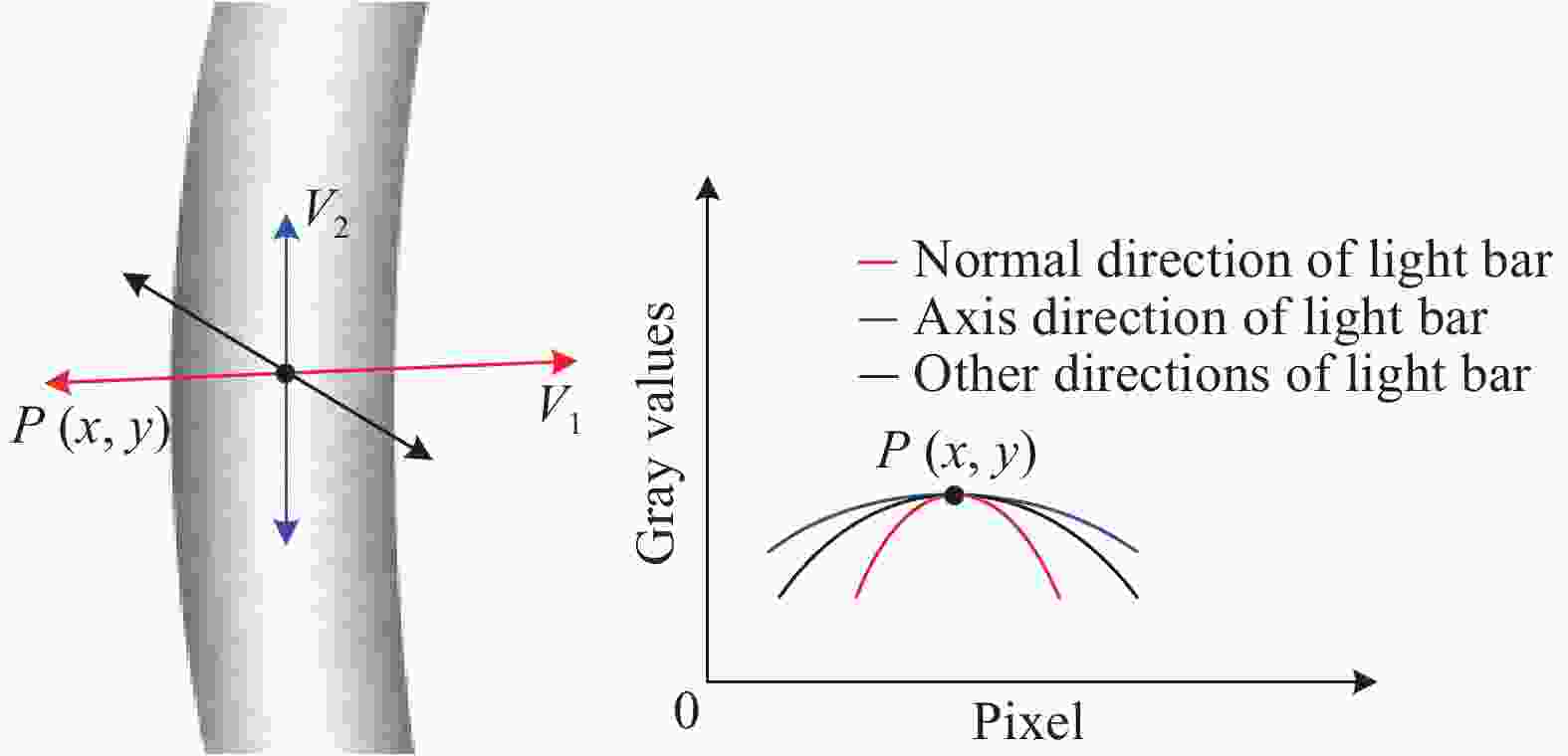
图 7 Hessian矩阵的特征值和特征向量表征示意图
Figure 7. Eigenvalues and eigenvectors of Hessian matrix
图7中
$P\left( {x,y} \right)$ 点为光条的精确中心点,基于上述方法,实现整段光条精确中心点群的提取,形成条状曲线段。对图6畸变光栅图像中心线条纹提取,提取前后对比示意图如下图8所示。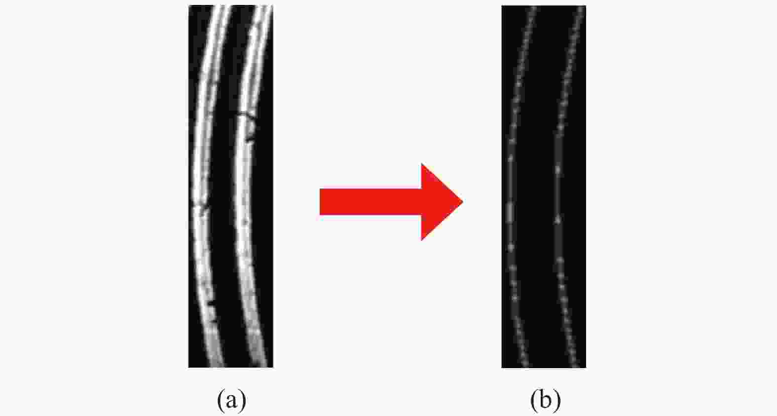
图 8 畸变光栅图像(a)及中心线提取后图像(b)
Figure 8. Distorted grating image (a) and center lines image (b)
-
畸变光栅图像实现中心线条纹有效提取后,施加多条等间隔水平参考线,参考线与纵向光栅中心线交点为特征点,如图9所示。

图 9 特征点
Figure 9. Feature points
为了实现畸变光栅图像水平方向的位移校正,需设置纵向参考线,对每一条中心线条纹上的特征点横坐标进行算术平均,从而获取纵向参考线横坐标数值,如图10所示。

图 10 中心线及纵向参考线
Figure 10. Center lines and reference lines
-
在整幅光栅图像中,每条纵向光栅条纹都有对应的纵向参考线,对图像任一行而言,光栅条纹中心线上特征点与对应的纵向参考线之间都存在像素水平位移量
$\Delta {S_i}$ ,如图11所示。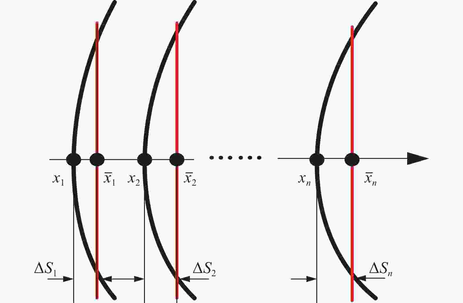
图 11 像素水平位移校正量示意图
Figure 11. Horizontal displacement correction
$$ \Delta {S_i} = {x_i} - {\bar x_i},\;i = 1,2, \cdots ,n $$ 通过上述公式计算得出的
$n$ 组数据$\left( {{x_i},\Delta {S_i}} \right)$ ,由于图像中各像素点在水平方向均存在畸变,因此采用基于最小二乘法的$n$ 次多项式插值方法,对已知数据展开拟合,能够获取每个像素点对应的水平方向位移量。通过比较不同次数多项式插值拟合结果的拟合度、拟合误差以及运算效率,筛选出校正决定系数(用于评价拟合近似程度)较高、均方根误差值较低,且运算效率较高的最优次数的多项式插值方法,得到水平方向像素畸变校正矩阵。纵向畸变校正方法与横向畸变校正方法类似,在水平方向畸变校正之后,基于Hessian矩阵对横向畸变光栅图像提取光栅中心线,拾取特征点并设置横向参考线,再次采用基于最小二乘法的
$n$ 次多项式插值方法,对已知数据进行拟合,得出每个像素点的竖直方向位移量,筛选出最优次数的多项式插值方法,得到竖直方向像素畸变校正矩阵,最终实现图像二维畸变校正。在图像二维畸变校正过程中,原图相邻像素若畸变校正量不同会产生间隙像素,灰度值为0,破坏图像清晰度和完整性,如图12所示。

图 12 畸变校正后间隙像素示意图
Figure 12. Gap pixels after distortion corrections
因此,可采用加权平均法填补间隙像素灰度值,最大程度还原图像信息。设原相邻两像素分别为
${H_m}$ 和${H_{m + 1}}$ ,像素灰度值分别为${R_m}$ 和${R_{m + 1}}$ ,中间形成了$n$ 个间隙像素,分别为像素${N_1},{N_2}, \cdots ,{N_n}$ ,则间隙像素${N_i}$ 的灰度值为:$$ {R_i} = \dfrac{{n - i + 1}}{{n + 1}}{R_m} + \dfrac{i}{{n + 1}}{R_{m + 1}},\left( {i = 1,2, \cdots ,n} \right) $$ -
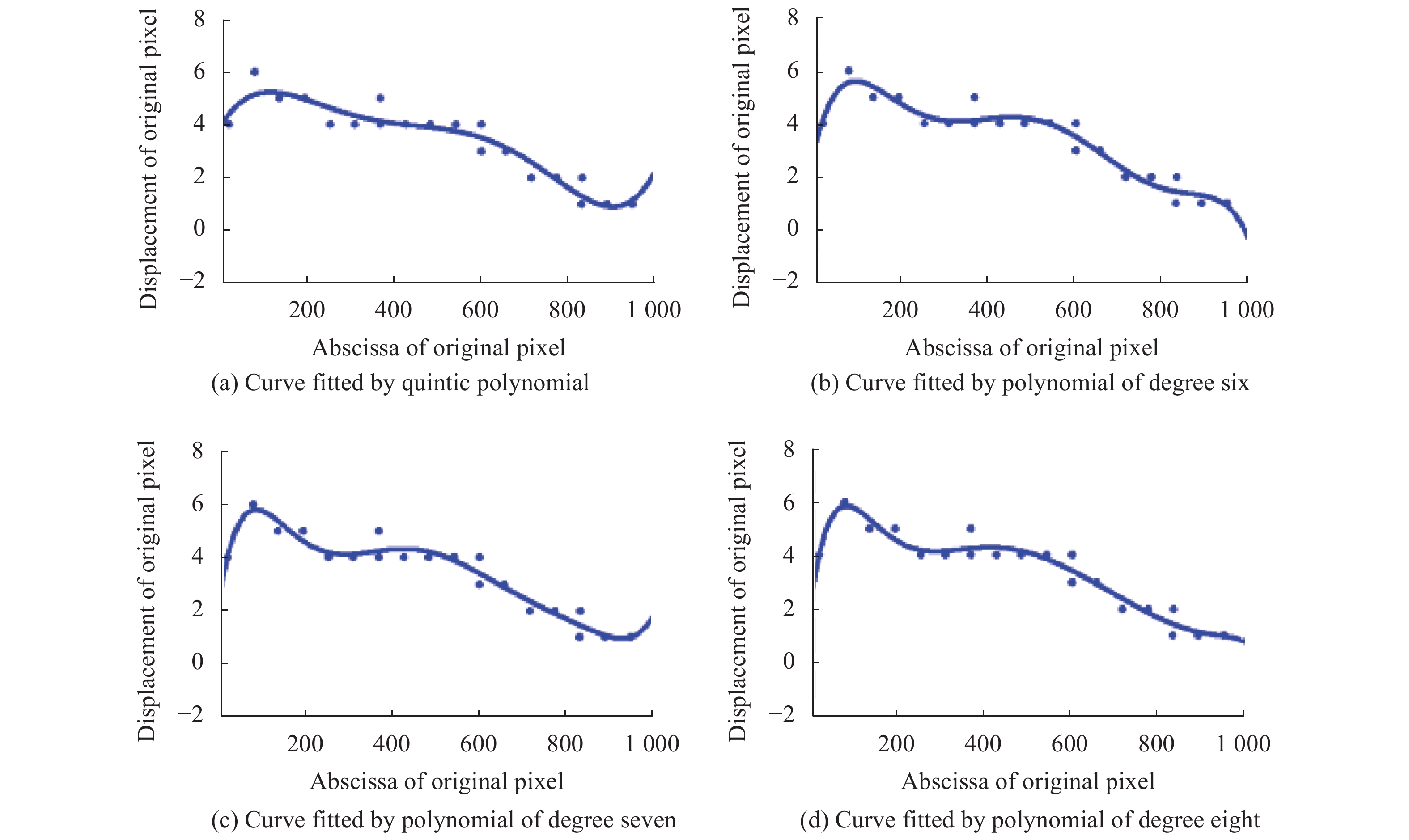
为验证上述图像畸变校正方法的可行性及有效性,对畸变光栅图像(图6)进行图像畸变校正。采用基于最小二乘法的多项式插值法,实现像素水平位移量的插值拟合,随机采样图像某一行数据(例如:第300行),分别采用5次多项式、6次多项式、7次多项式以及8次多项式进行插值拟合,插值结果如图13所示,计算如下:
$$\left\{ {\begin{array}{*{20}{l}} {p\left( x \right) = 2.1{{\rm{e}}^{ - 13}}{x^5} - 5.2{{\rm{e}}^{ - 10}}{x^4} + 4.6{{\rm{e}}^{ - 7}}{x^3} - 1.8{{\rm{e}}^{ - 4}}{x^2} + 2.5{{\rm{e}}^{ - 2}}x + 4.0} \\ {p\left( x \right) = - 9.1{{\rm{e}}^{ - 16}}{x^6} + 2.9{{\rm{e}}^{ - 12}}{x^5} - 3.6{{\rm{e}}^{ - 9}}{x^4} + 2{{\rm{e}}^{ - 6}}{x^3} - 5.7{{\rm{e}}^{ - 4}}{x^2} + 6.3{{\rm{e}}^{ - 2}}x + 3.3} \\ {p\left( x \right) = 1.9{{\rm{e}}^{ - 18}}{x^7} - 7.4{{\rm{e}}^{ - 15}}{x^6} + 1.9{{\rm{e}}^{ - 11}}{x^5} - 9.7{{\rm{e}}^{ - 9}}{x^4} + 4.3{{\rm{e}}^{ - 6}}{x^3} - 9.7{{\rm{e}}^{ - 4}}{x^2} + 9.2{{\rm{e}}^{ - 2}}x + 2.8} \\ {p\left( x \right) = - 2.3{{\rm{e}}^{ - 21}}{x^8} + 1.1{{\rm{e}}^{ - 17}}{x^7} - 2.2{{\rm{e}}^{ - 14}}{x^6} + 2.5{{\rm{e}}^{ - 11}}{x^5} - 1.6{{\rm{e}}^{ - 8}}{x^4} + 5.9{{\rm{e}}^{ - 6}}{x^3} - 1.2{{\rm{e}}^{ - 3}}{x^2} + 0.1x + 2.6} \end{array} } \right.$$ 
图 13 像素水平位移量多项式拟合曲线
Figure 13. Polynomial fitting curve of pixel horizontal displacement
通过上述计算结果及拟合曲线分析可知,5次、6次、7次以及8次多项式插值拟合校正决定系数分别为0.8737、0.9046、0.9078以及0.9003;均方根误差分别为0.5209、0.4525、0.4449以及0.4626;通过统计发现上述多项式插值运算时长基本相同。因此,7次项插值拟合校正决定系数最高,且均方根误差最小,为了进一步验证该结果有效性,对整幅图像512行分别进行5次、6次、7次以及8次多项式插值拟合,统计各次数多项式插值拟合为最优时占据的行数,如图14所示,7次项最优占379行,比例为
$74\% $ ,明显优于其他次数插值拟合,因此,认为7次项插值拟合最优。
图 14 多次项插值拟合最优情况统计
Figure 14. Statistics of multiple interpolation fitting
竖直方向也采用7次项插值拟合的方法进行畸变校正,最终二维畸变校正后光栅图像及中心线提取后图像如图15所示。

图 15 二维畸变校正后光栅图像(a)及中心线提取后图像(b)
Figure 15. Grating image after 2-D corrections (a) and center lines (b)
-
为了更精确评价畸变校正结果准确性,采用50 μm间距的网格畸变测试靶进行二维扫描成像,记录原始畸变图像,如图16(a)所示,通过上述方法实现二维畸变校正。将校正后图像与标准网格畸变测试靶图像进行对比,分析校正后二维方向的残差,并统计出最大、最小以及平均残差,图像局部放大后的残差分析示意图如图16(b)所示。

图 16 网格测试靶畸变图像(a);畸变校正后网格图像(b)
Figure 16. Distorted image of grid test target (a); Grid image after distortion correction (b)
畸变矫正后的网格畸变测试靶与标准网格畸变测试靶二维方向上残差最大为4个像素,最小为0个像素,平均为1.15个像素,由于像素数实际为整数,因此,近似认为平均残差约1个像素。
-
在当前存在畸变的系统中开展在体皮肤共聚焦成像实验,记录皮肤组织结构特征较为明显的棘层图像。校正前后对比如图17所示,能够明显看出,皮肤棘层细胞结构形态由原先的斜拉伸状变为较为均匀的蜂窝状,能够清晰辨识正常组织特征,有利于皮肤组织结构信息准确获取,辅助医生检测和诊断。

图 17 皮肤棘层图像畸变校正前后对比
Figure 17. Contrast of skin echinoderm images before and after distortion correction
-
文中2.2节已分析出MEMS振镜扫描畸变模型及对应的表达式,可推算出真实图像中各像素点对应的准确扫描角度
$\alpha $ 、$ \;\beta$ ,而扫描角度与控制电压呈固定关系,因此能够得出各像素点与控制电压的一一映射关系,理论上MEMS振镜只需读取准确的控制电压矩阵即可生成完全无畸变图像。但在实验时发现该方法计算量庞大,且这种外部数据读取的方式直接影响MEMS振镜扫描速度,从而影响系统成像速度,无法满足在体实时成像要求。而文中畸变校正方法具有一定的普适性和通用性,不受畸变模型限制,虽然多次项插值拟合方式的校正精度与之相比略低,但已基本不影响图像的观察和分析,且该方法不会影响系统成像速度,完全满足使用要求。
-
文中针对单镜面型MEMS振镜开展了二维扫描畸变机理分析,提出一种有效的的二维畸变校正算法,实现图像畸变准确校正。首先记录原始光栅畸变图像,然后基于Hessian矩阵提取光栅中心线,拾取特征点并设置基准参考线,通过基于最小二乘法的7次多项式插值法标定二维方向像素畸变校正量,最终实现图像畸变校正。利用网格畸变测试靶进行残差分析,二维方向上残差最大为4个像素,最小为0个像素,平均为1.15个像素,校正结果较为精确。皮肤在体实时成像实验显示,图像畸变校正后组织结构特征更加真实准确,表明这种校正算法有效可行,有助于皮肤疾病的准确诊断。
Analysis and correction of image distortion in MEMS galvanometer scanning confocal system
-
摘要: 在皮肤反射式共聚焦显微成像过程中,针对MEMS振镜二维扫描引起的共聚焦图像畸变,开展了光束偏转理论分析,得出了投影面扫描图像的具体形状表征,理论畸变图像与真实畸变图像一致,明确了畸变机理,提出一种有效的畸变校正算法,实现对图像二维畸变的校正。首先记录原始光栅畸变图像,然后基于Hessian矩阵提取光栅中心线,拾取特征点并设置基准参考线,通过基于最小二乘法的7次多项式插值法标定二维方向像素畸变校正量,采用加权平均法填补间隙像素灰度值,最终实现图像畸变校正。利用网格畸变测试靶实验得出7次多项式插值后的校正决定系数最高、均方根误差值最低,整幅512行图像在7次多项式插值后最优行数占379行,比例为74%,通过残差分析,二维方向上残差最大为4个像素,最小为0个像素,平均为1.15个像素,校正结果较为精确。皮肤在体实时成像实验显示,图像畸变校正后组织结构特征更加真实准确,表明这种校正算法有效可行,有助于皮肤疾病的准确诊断。Abstract: Aiming at the distorted confocal images caused by the two-dimensional scanning of MEMS galvanometer during skin imaging by reflectance confocal microscopy, the theoretical analysis of beam deflection was carried out, and the specific shape representation of projection plane scanning image was obtained. It was concluded that the theoretical distortion image was consistent with the real distortion image. The distortion mechanism was clarified and a distortion correction method was proposed. First, the original distorted grating image was recorded, then the center lines of grating were obtained based on the Hessian matrix, after that feature points were picked and datum reference lines were set. Finally, the correction to the distorted confocal images was realized by calibrating the corrections of the two-dimensional pixel distortions using polynomial interpolation based on the least square method and filling the gray value of gap pixels by weighted average method. By the experiment of measuring target with grid distortion, the correction coefficient was the highest and the root mean square error was the lowest after polynomial interpolation of degree 7. Also, the optimal number of 512 rows was 379, accounting for 74%. The residual distortions were accurately evaluated, in two dimensional, the maximum value is 4 pixels, the minimum value was 0 pixel and the average value was 1.15 pixels, so the results were accurate. The experiment of in vivo real-time skin imaging shows that the organizational structure features are more real and accurate after corrections. So this method is effective and feasible, which is helpful for accurate diagnosis of skin diseases.
-
图 8 畸变光栅图像(a)及中心线提取后图像(b)
Figure 8. Distorted grating image (a) and center lines image (b)
图 13 像素水平位移量多项式拟合曲线
Figure 13. Polynomial fitting curve of pixel horizontal displacement
图 15 二维畸变校正后光栅图像(a)及中心线提取后图像(b)
Figure 15. Grating image after 2-D corrections (a) and center lines (b)
图 16 网格测试靶畸变图像(a);畸变校正后网格图像(b)
Figure 16. Distorted image of grid test target (a); Grid image after distortion correction (b)
-
[1] 刘创, 张运海, 黄维, 等. 皮肤反射式共聚焦显微成像扫描畸变校正[J]. 红外与激光工程, 2018, 47(10): 1041003. Liu Chuang, Zhang Yunhai, Huang Wei, et al. Correction of reflectance confocal microscopy for skin imaging distortion due to scan [J]. Infrared and Laser Engineering, 2018, 47(10): 1041003. (in Chinese) [2] 肖昀, 张运海, 王真, 等. 入射激光对激光扫描共聚焦显振镜分辨率的影响[J]. 光学 精密工程, 2014, 22(1): 31-38. doi: 10.3788/OPE.20142201.0031 Xiao Yun, Zhang Yunhai, Wang Zhen, et al. Effect of incident laser on resolution of LSCM [J]. Optics and Precision Engineering, 2014, 22(1): 31-38. (in Chinese) doi: 10.3788/OPE.20142201.0031 [3] 郑亚杰, 沈雪, 崔勇. 皮肤镜联合反射式共聚焦显振镜对色素痣良恶性、脂溢性角化病的诊断价值[J]. 中日友好医院学报, 2018, 32(2): 79-82, 64. Zheng Yajie, Shen Xue, Cui Yong. Diagnostic value of reflectance confocal microscopy combined with dermoscopy onbenign and malignant melanocytic nevus and seborrheic keratosis [J]. Journal of China-Japan Friendship Hospital, 2018, 32(2): 79-82, 64. (in Chinese) [4] 朱宜彬. 反射式共聚焦激光扫描显微镜在皮肤科的应用研究[J]. 名医, 2018, 64(9): 136. Zhu Yibin. Application of reflective confocal laser scanning microscope in dermatology [J]. Renowned Doctor, 2018, 64(9): 136. (in Chinese) [5] 刘才明. 激光大屏幕显示系统中振镜扫描的工作原理及图像失真研究[J]. 中国激光, 2003, 12(3): 263-266. doi: 10.3321/j.issn:0258-7025.2003.03.018 Liu Caiming. Study on the working principle and image distortion of galvanometer scanning in laser large screen display system [J]. Chinese Journal of Lasers, 2003, 12(3): 263-266. (in Chinese) doi: 10.3321/j.issn:0258-7025.2003.03.018 [6] Jiang Ming, Yu Jianhua, Luo Xiaoling, et al. Study on graphic distortion in laser display [J]. Chinese Journal of Lasers, 1999, 8(6): 509-512. [7] 陈方杰, 韩军, 王祖武, 等. 基于改进GMS和加权投影变换的图像配准算法[J]. 激光与光电子学进展, 2018, 55(11): 111006. Chen Fangjie, Han Jun, Wang Zuwu, et al. Image registration algorithm based on improved GMS and weighted projection transformation [J]. Laser & Optoelectronics Progress, 2018, 55(11): 111006. (in Chinese) [8] 魏启元, 吕晓琪, 谷宇. 改进投影变换和保留结构特征的拼接图像修复算法[J]. 现代电子技术, 2017, 40(23): 38-42, 46. Wei Qiyuan, LV Xiaoqi, Gu Yu. Improved projection transformation and structural feature preserving mosaic image restoration algorithm [J]. Modern Electronic Technology, 2017, 40(23): 38-42, 46. (in Chinese) [9] 樊城城. 基于投影变换多元统计控制模型的改进[D]. 苏州: 苏州大学, 2017. Fan Chengcheng. Improvement of multivariate statistical control model based on projection transformation[D]. Suzhou: Soochow University, 2017. (in Chinese) [10] Anatoliy Kovalchuk, Ivan Izonin, Mihal Gregush ml, et al. An efficient image encryption scheme using projective transformations [J]. Procedia Computer Science, 2019, 160: 584-589. [11] 黄明益, 吴军. 理想投影椭圆约束下的鱼眼镜头内部参数标定[J]. 中国图象图形学报, 2019, 24(11): 1972-1984. doi: 10.11834/jig.190061 Huang Mingyi, Wu Jun. internal parameter calibration of fish eye lens under the constraint of ideal projection ellipse [J]. Journal of Image and Graphics, 2019, 24(11): 1972-1984. (in Chinese) doi: 10.11834/jig.190061 [12] 远国勤, 郑丽娜, 张洪文, 等. 线阵相机二维高精度内方位元素标定[J]. 光学 精密工程, 2019, 27(8): 1901-1907. doi: 10.3788/OPE.20192708.1901 Yuan Guoqin, Zheng Li'na, Zhang Hongwen, et al. Two dimensional high-precision internal orientation element calibration of linear array camera [J]. Optical & Precision Engineering, 2019, 27(8): 1901-1907. (in Chinese) doi: 10.3788/OPE.20192708.1901 [13] 王向军, 白皓月, 吴凡璐, 等. 基于改进球面透视投影的鱼眼图像畸变校正方法[J]. 图学学报, 2018, 39(1): 43-49. Wang Xiangjun, Bai Haoyue, Wu Fanlu, et al. Fish eye image distortion correction method based on improved spherical perspective projection [J]. Journal of Graphics, 2018, 39(1): 43-49. (in Chinese) [14] Zhang Baofeng, Qi Zhiqiang, Zhu Junchao, et al. Omnidirection image restoration based on spherical perspective projection[C]//APCCAS 2008, 2008. [15] 王依桌. 鱼眼图像的校正与柱面全景拼接方法[D]. 哈尔滨: 哈尔滨工程大学, 2013. Wang Yizhuo. Correction of fisheye image and mosaic method of cylindrical panorama[D]. Harbin: Harbin Engineering University, 2013. (in Chinese) [16] 刘亿静, 苗长云, 杨彦利. 基于经纬映射的径向畸变快速校正算法的研究[J]. 激光杂志, 2015, 36(1): 1-4. Liu Yijing, Miao Changyun, Yang Yanli. Research on fast correction algorithm of radial distortion based on longitude latitude mapping [J]. Laser Journal, 2015, 36(1): 1-4. (in Chinese) [17] 魏利胜, 周圣文, 张平改, 等. 基于双经度模型的鱼眼图像畸变矫正方法[J]. 仪器仪表学报, 2015, 36(2): 377-385. Wei Lisheng, Zhou Shengwen, Zhang Pinggai, et al. Correction method of fish eye image distortion based on double longitude model [J]. Chinese Journal of Scientific Instrument, 2015, 36(2): 377-385. (in Chinese) [18] 肖潇, 王伟, 毕凯. 柱面透视投影模型下的全景环形透镜畸变校正[J]. 西安电子科技大学学报, 2013, 40(1): 87-92. Xiao Xiao, Wang Wei, Bi Kai. Distortion correction of panoramic circular lens under cylindrical perspective projection model [J]. Journal of Xidian University , 2013, 40(1): 87-92. (in Chinese) [19] 周辉, 罗飞, 李慧娟, 等. 基于柱面模型的鱼眼影像校正方法的研究[J]. 计算机应用, 2008, 28(10): 2664-2666. Zhou Hui, Luo Fei, Li Huijuan, et al. Research on correction method of fish eye image based on cylinder model [J]. Computer Application, 2008, 28(10): 2664-2666. (in Chinese) [20] Tsai R Y. A versatile camera calibration technique for high accuracy SD machine vision metrology using off-the-shelf TVcameras and lenses [J]. IEEE Jourmal of Robotics Automation, 1987, 3(4): 323-344. doi: 10.1109/JRA.1987.1087109 [21] Zhang Z. A flexible new technique for camera calibration [J]. IEEE Transactions on Pattern Analysis and Machine Intelligence, 2000, 22(11): 1330-1334. doi: 10.1109/34.888718 [22] 何亚洲. 基于机器学习的图像畸变校正及测温误差分析[D]. 大连: 大连理工大学, 2018. He Yazhou. Image distortion correction and temperature measurement error analysis based on machine learning[D]. Dalian: Dalian University of Technology, 2018. (in Chinese) [23] 韩黄璞. 基于成像规律的CCD镜头畸变的快速校正[D]. 西安: 西安工业大学, 2012. Han Huangpu. Fast correction of CCD lens distortion based on imaging law[D]. Xi'an: Xi'an Technological University, 2012. (in Chinese) [24] 王岚, 李新华. 基于改进遗传模拟退火算法的BP神经网络的畸变校正研究[J]. 计算机测量与控制, 2019, 27(5): 77-81. Wang Lan, Li Xinhua. Distortion correction of BP neural network based on improved genetic simulated annealing algorithm [J]. Computer Measurement & Control, 2019, 27(5): 77-81. (in Chinese) -

 点击查看大图

计量
- 文章访问数: 582
- HTML全文浏览量: 183
- PDF下载量: 99
- 被引次数: 0


