


-
目标检测是进行场景内容理解等高级视觉任务的前提,已广泛应用于智能视频监控、基于内容的图像检索、视觉导航等任务中。传统的目标检测主要使用人工设计的特征(如HAAR[1]、HOG[2]、SHIFT[3]、SURF[4]等),在滑动窗口下使用分类器进行判别,其代表方法有Adaboost-SVM[5]和形变部件模型(DPM)[6-8]。上述方法开创了实用化的目标检测之先河,在便携式设备和机器人等领域有着广泛应用。但由于人工设计特征的性能所限,传统方法的准确率始终不高,且通常对新的图像缺乏足够的泛化能力。
相比传统目标检测方法,基于卷积神经网络(CNN)的目标检测方法在准确率方面具有显著优势。CNN通过大量参数拟合各类不同的情形,使用多层架构逐步抽象目标信息,极大地提升了目标检测的泛化能力。然而当前基于CNN的目标检测相关研究集中于RGB图像等多通道图像,而对红外目标检测的研究相对较少。另一方面,红外目标检测领域的相关研究多为针对特定类型目标(例如火灾[9])的检测识别,或弱小目标检测[10],而在多分类红外目标检测方面依然欠缺。
基于CNN的目标检测架构可分为两大模块:CNN主干网络(Backbone)和检测器网络(Detector),其中CNN主干网络主要用于多层特征提取,检测器主要负责输出目标位置及其类别。由于红外图像与RGB等多通道图像的最大区别在于图像特征层面,红外目标检测的关键在于优化CNN主干网络,检测器部分则可采用Faster R-CNN[11]、R-FCN[12]、YOLO[13]、SSD[14]等现有方法。相比于RGB图像,红外图像有两大特点:其一,标注数据不足,训练样本相对较少;其二,红外图像的纹理信息远少于RGB图像。上述特点决定了CNN在红外图像中所能有效训练的参数数量远低于RGB图像,因此需要通过约束和在线剪枝剔除冗余参数,避免过拟合。考虑到对网络权重进行Lp归一化能够有效控制神经网络的稀疏性,文中提出了一种使用Lp归一化权重的红外目标检测网络压缩方法,主要用于改进基于CNN的目标检测架构在红外目标检测上的适应性,在压缩网络规模的同时提升其泛化能力。实验结果表明该方法显著降低了红外目标检测网络的权重数目,同时提升了红外目标检测测试精度,验证了所提出方法的有效性。
-
给定L层神经网络,其每个神经元的权重被约束在单位Lp球面上,该神经网络模型为:
$$\begin{array}{l} {\hat{\boldsymbol y}} = f({\boldsymbol{x}};\vartheta ), \\ {\rm{s.t.}}\quad ||{\boldsymbol{w}}_j^{(l)}|{|_{{p^{(l)}}}} = 1,l = 1,2, \cdots ,L,j = 1,2, \cdots ,{J^{(l)}}, \\ \end{array} $$ (1) 式中:x为网络输入;
${\hat{\boldsymbol y}}$ 为网络输出;$\vartheta = \{ {\boldsymbol{w}},b\} $ 为网络的权重和偏置的集合;${{\boldsymbol{w}}_j}^{(l)}$ 表示l层的第j个权重;$b_j^{(l)}$ 为对应的偏置项;$||{\boldsymbol{w}}|{|_p} = 1$ 表示神经元的权重被约束在单位Lp球面上,即对其进行Lp归一化。为了说明为权重引入Lp归一化的意义,首先阐述该约束对神经网络的权重稀疏性的影响,而受约束神经网络的训练方法将在下一节予以介绍。
图1所示为公式(1)所定义网络的某个神经元的权重分布随p的变化,其中横坐标为p,纵坐标为权重序号,其每一列表示特定p下的权重分布,越亮的部分权重幅度越大。可以观察到随着p的增大,权重分布变得越来越稠密。该现象说明网络的稀疏性可以通过p进行控制。由于图中黑色部分的权重很小且接近于0,这些权重可以被安全地移除而不影响网络的准确性,从而实现神经网络的稀疏化。
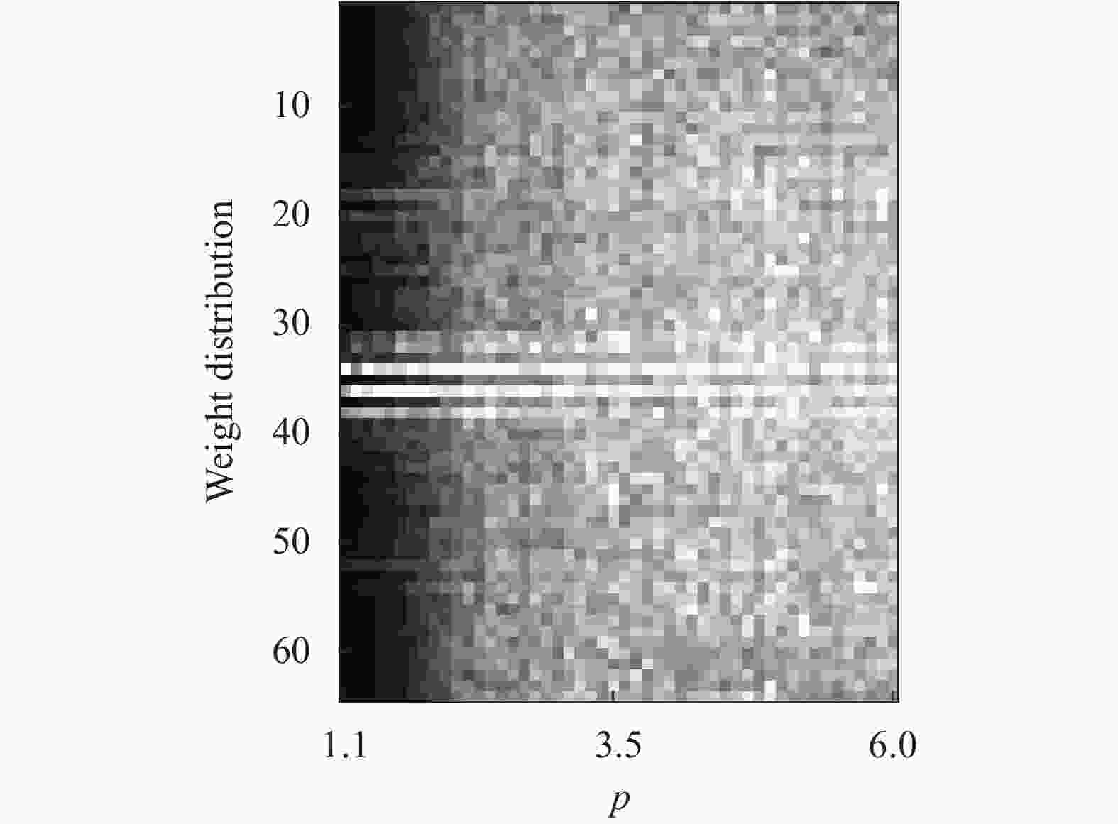
图 1 单个神经元权重分布随p的变化
Figure 1. Weight distribution of a neuron with respect to p
为了量化评估网络权重的稀疏性与p之间的关系,在Fashion-MNIST数据集上测试有监督训练下公式(1)所定义CNN的三个卷积层的权重稀疏性随p的变化,结果如图2所示。容易发现卷积层的权重稀疏性与p有着显著的负相关关系,且不同卷积层所遵循的规律高度一致,说明通过调节p能够精确地控制网络各层的权重稀疏性。基于这一规律,文中设计了目标检测网络稀疏化训练方法,下面予以介绍。

图 2 卷积层权重稀疏性随p的变化
Figure 2. Sparsity of weight with respect to p at convolutional layers
-
当前主流的目标检测模型,无论是单阶段目标检测(Single stage object detector)还是两阶段目标检测(Two-stage object detector),可大体上分为两大部分:负责特征提取的CNN主干网络(Backbone)与负责输出目标位置和类别的检测器网络(Detector)。通常情况下,主干网络相比检测器参数数目更多,模型规模更大,故对主干网络进行稀疏化能够有效压缩目标检测模型规模。另一方面,检测器中的边框回归(Bounding-box regression)与分类器(Classifier)对权重的总体幅度较为敏感,不适合采用Lp归一化的权重。综合上述因素,文中所用目标检测器的训练流程如图3所示,其中主干网络以及邻接的Neck模块使用文中提出的Lp球面梯度下降法(LpSGD)进行训练,将特征提取网络权重稀疏化;目标检测器及其附属部分使用经典的梯度下降法(SGD)训练,以保证边框回归和分类器的精度。

图 3 目标检测网络稀疏化训练流程
Figure 3. Training process of sparse neural network for object detection
-
记
$\vartheta = \{ {\boldsymbol{w}}_j^{(l)},{b_j},l = 1,2, \cdots ,L,j = 1,2, \cdots ,{J^{(l)}}\} $ 表示网络各层权重与偏置的集合,则公式(1)所定义的网络可通过约束条件下的经验风险最小化(Empirical Risk Minimization, ERM)进行训练:$$\begin{array}{l} \mathop {\min }\limits_\vartheta R = \dfrac{1}{n}\displaystyle\sum\limits_{i = 1}^n {{\mathcal{L}}\left( {{{{\hat{\boldsymbol y}}}_i},{{\boldsymbol{y}}_i}} \right)} \\ {\rm{s.t.}}\quad {\left\| {{\boldsymbol{w}}_j^{(l)}} \right\|_{{p^{(l)}}}} = 1,l = 1,2, \cdots ,L,j = 1,2, \cdots ,{m^{(l)}} \\ \end{array} $$ (2) 式中:
${\mathcal{L}}\left( {{{{\hat{\boldsymbol y}}}_i},{{\boldsymbol{y}}_i}} \right)$ 表示网络关于第i个训练样本预测值的损失函数(Loss function),${{\hat{\boldsymbol y}}_i}$ 和${{{\boldsymbol{y}}_i}} $ 分别为网络输出的预测值和标注值。对应的增广ERM为:
$$\mathop {\min }\limits_\vartheta {R^*} = R + \sum\limits_{l = 1}^L {\sum\limits_j {\frac{{\lambda _j^{(l)}}}{{{p^{(l)}}}}(||{{\boldsymbol{w}}_j}^{(l)}||_{{p^{(l)}}}^{{p^{(l)}}} - 1)} } $$ (3) 式中:
$\lambda _j^{(l)}$ 为关于${{\boldsymbol{w}}_j}^{(l)}$ 归一化约束的拉格朗日乘子(Lagrange multiplier),同时为${{\boldsymbol{w}}_j}^{(l)}$ 的归一化系数。对公式(3)求关于
${{\boldsymbol{w}}_j}^{(l)}$ 的导数,得到方程:$$\lambda _j^{(l)}{\left( {{{\boldsymbol{w}}_j}^{(l)}} \right)^{[{p^{(l)}} - 1]}} = - {\nabla _{{{\boldsymbol{w}}_j}^{(l)}}}R\left( {{{\boldsymbol{w}}_j}^{(l)}} \right),l = 1,2, \cdots ,L$$ (4) $ {\nabla _{\boldsymbol{w}}}R $ 表示$R$ 关于w的梯度,${\left( {{{\boldsymbol{w}}_j}^{(l)}} \right)^{[{p^{(l)}} - 1]}}$ 满足:$${{\boldsymbol{w}}^{[p]}} = {\rm{sgn}} ({\boldsymbol{w}}) \circ |{\boldsymbol{w}}{|^p}$$ (5) 表示向量w每个元素的p次幂乘以其对应符号,即
${{\boldsymbol{w}}^{[p]}}$ 的每个元素满足$w_j^{[p]} = {\rm{sgn}} ({w_j})|{w_j}{|^p}$ 。为了对
${\boldsymbol{w}}$ 进行Lp归一化,$\lambda _j^{(l)}$ 应满足:$$\lambda _j^{(l)} = {\left\| {{\nabla _{{\boldsymbol{w}}_j^{(l)}}}R\left( {{\boldsymbol{w}}_j^{(l)}} \right)} \right\|_q}$$ (6) 式中:
$q = p/(p - 1) $ 。记:
$$\Delta ({\boldsymbol{w}}) = {\left[ {\frac{{{\nabla _{\boldsymbol{w}}}R({\boldsymbol{w}})}}{\lambda }} \right]^{[q - 1]}}$$ (7) 为权重w的特征函数。将公式(7)代入公式(4)得到最优权重应当满足:
$${{\boldsymbol{w}}_j}^{(l)} = - \Delta ({{\boldsymbol{w}}_j}^{(l)})$$ (8) 设权重的更新率为η,将公式(8)展开表示为:
$${{\boldsymbol{w}}_j}^{(l)} = (1 - \eta ){{\boldsymbol{w}}_j}^{(l)} - \eta \Delta ({{\boldsymbol{w}}_j}^{(l)})$$ (9) 得到
$t + 1$ 次迭代的权重满足:$${{\boldsymbol{w}}_j}^{(l,t + 1)} = \frac{1}{{\rho _j^{(l,t + 1)}}}\left[ {(1 - \eta ){{\boldsymbol{w}}_j}^{(l,t)} - \eta \Delta ({{\boldsymbol{w}}_j}^{(l,t)})} \right]$$ (10) 式中:
$\;\rho _j^{(l,t + 1)} = {\left\| {(1 - \eta ){{\boldsymbol{w}}_j}^{(l,t)} - \eta \Delta ({{\boldsymbol{w}}_j}^{(l,t)})} \right\|_{{q^{(l)}}}}$ 表示${{\boldsymbol{w}}_j}^{(l,t + 1)}$ 的归一化系数;${{\boldsymbol{w}}_j}^{(l,t)}$ 与${{\boldsymbol{w}}_j}^{(l,t + 1)}$ 分别表示${{\boldsymbol{w}}_j}^{(l)}$ 在第t次和第$t + 1$ 次迭代的值。随后,每隔若干次迭代将各个神经元中绝对值小于阈值(接近于0)的权重进行剪枝,从而将神经网络稀疏化。
偏置的更新率与权重更新率保持一致,但使用经典梯度下降予以优化:
$${b_j}^{(l,t + 1)} = {b_j}^{(l,t)} - \eta \;{\nabla _{{b_j}^{(l)}}}R({b_j}^{(l,t)})$$ (11) 式中:
${\nabla _{{b_j}^{(l)}}}R({b_j}^{(l,t)})$ 是经验损失函数关于偏置${b_j}^{(l)}$ 的梯度。LpSGD的伪代码见算法1。需要说明的是,由于神经网络的参数规模相对数据集常常是过拟合的,Lp归一化既能压缩网络规模,又能提升其泛化能力。另外,LpSGD可以方便的与Momentum、RMSprop、Adam等方法相结合,从而为公式(1)所定义的受约束模型提供多样化的训练方法。
算法1: LpSGD
Algorithm 1: LpSGD
Input: Neural network (1), dataset with inputs {x1,···, xn} and label {y1,···, yn}, Update ratio η, norm parameter p(l), l = 1,···, L, topology evolution frequency T, BatchSize, Epoches.
Output: Parameters of network
$\vartheta = \{ {\boldsymbol{w}}_j^{(l)},b_j^{(l)},l = $ $ 1, \cdots , L,j = 1, \cdots ,{J^{(l)}}\} $ 1. Initialize parameters of neural network
$\vartheta $ , and the feature function of weights defined in function (1);2. FOR Each Epoch
3. FOR Each Batch
4. Sampling BatchSize number of data form training dataset;
5. FOR l=1, ···, L
6. Update weight with function (10);
7. Update bias with funciton (11);
8. IF batchNumber is divisible by T
9. Drop the connection whose weight close to zero;
10. END IF
11. END FOR
12. END FOR
13. END FOR
-
为对比稠密目标检测网络和稀疏目标检测网络的性能,文中选用包含四类目标的小规模红外仿真数据集进行算法验证。该数据集由实验室开发的红外仿真生成软件生成,共包含942个标注物体,其中829个为训练样本,113个为测试样本,数据集的详细统计信息如表1所示。实验使用Faster R-CNN、SSD300、YOLOv3作为基准模型,上述三个模型首先在训练集上分别进行50、70、105个Epoch的训练,随后在测试集中验证其精度。实验硬件环境为Nvidia TITAN X GPU,Intel Exon E5-2667 CPU;软件环境为Unbuntu 16.04,Pytorch 1.5,Mdetection 2。
表 1 红外仿真数据集
Table 1. Simulated infrared dataset
Classification Training Test Total Class 1 208 28 236 Class 2 210 26 236 Class 3 219 30 249 Class 4 192 29 221 Total 829 113 942 实验中部分代表性的检测结果如图4所示,其中每行为同一幅图片使用不同方法的检测结果,第一列至第四列分别为Faster R-CNN、稀疏化Faster R-CNN、SSD300、稀疏SSD300,最后一列为标注(Ground truth)。可以看出在第一行中,四种方法的检测结果相当,定位和分类结果基本一致;第二行中,稀疏模型输出结果(g)、(i)的定位精度优于对应的稠密模型输出结果(f)、(h),且(i)修正了(h)中的一个漏检;第三行的结果中,稀疏SSD修正了稠密SSD的冗余边框(图4(m));第四行中,稀疏模型检测出的边框要比稠密模型更加紧凑,精度更高。

图 4 经典网络和稀疏化网络红外目标检测结果对比
Figure 4. Result comparison of infrared object detection between classical neural networks and sparse neural networks
下面从定量的角度评估稀疏网络相比于稠密网络的参数压缩比例及其准确率的变化。其中模型规模(Scale)使用非0参数数量评价,模型精度使用mAP表示,并在包含113个样本的测试集上验证各个模型的mAP。为了平衡模型参数数目与精度,稀疏网络的训练当中主干网络的前4层使用p = 1.3,后面所有层使用p = 1.15进行稀疏化,各个模型的有效参数的数目和检测精度如表2所示。
表 2 红外仿真数据集目标检测模型及其结果
Table 2. Object detection model and result on simulated infrared dataset
Method Scale AP mAP Backbone Detector Class 1 Class 2 Class 3 Class 4 Faster R-CNN Dense 26 852 416 14 511 140 0.912 0.885 0.927 0.972 0.925 Sparse 5 337 352 14 511 130 0.910 0.875 0.936 0.982 0.926 SSD300 Dense 22 943 936 1 202 958 0.893 0.879 0.914 0.965 0.914 Sparse 4 103 396 1 202 958 0.889 0.867 0.924 0.981 0.917 YOLOv3 Dense 55 294 688 6 245 196 0.914 0.898 0.919 0.972 0.926 Sparse 14 829 742 6 245 196 0.906 0.895 0.927 0.984 0.928 从表2中可以看到,无论对于Faster R-CNN、SSD还是YOLOv3而言,稀疏模型相比于稠密模型的有效参数数量均显著减少,同时mAP都有着少量提升。尤其是在SSD上,稀疏网络相比稠密网络参数的压缩比达到了78%,且mAP提升了0.3个百分点。相比于Faster R-CNN的稀疏化,SSD和YOLOv3的稀疏化无论是在参数压缩比还是精度方面都有着更加明显的优势,说明文中的稀疏化方法相比于两阶段模型而言更加适用于单阶段模型。究其原因在于SSD、YOLOv3这样的单阶段模型参数主要集中于主干网络当中,而Faster R-CNN这类的两阶段模型在Detector部分的Region Proposal Networks(RPN)上有着大量的参数,这些参数是不能够通过LpSGD算法进行稀疏化的,否则将极大地降低检测精度。关于mAP的少量提升,文中认为是稠密模型在数据集中过拟合,而稀疏化后模型规模减小使得过拟合程度减轻所致。另外,相比于Class 3和Class 4而言,Class 1与Class 2的图像更加复杂,故而网络稀疏化后造成了一定的特征损失,检测精度有所下降。
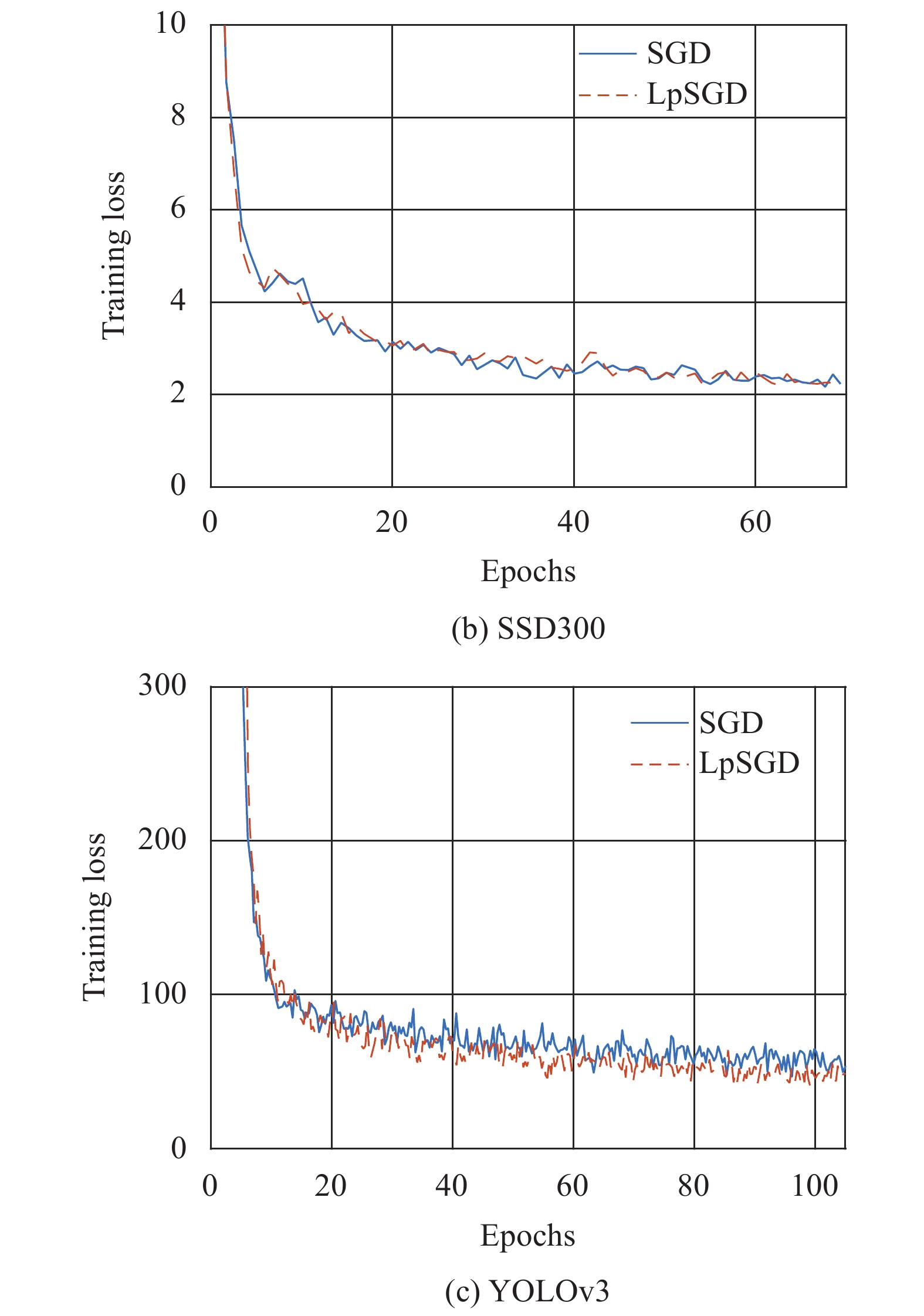
此外为了检验LpSGD算法收敛性,将红外仿真数据集上稠密网络和稀疏网络的收敛过程进行对比,如图5所示,其中图(a)~(c)分别展示了Faster R-CNN、SSD、YOLOv3的训练损失随迭代次数的变化。可以看到LpSGD与SGD训练过程当中的损失函数收敛过程基本一致,说明LpSGD与SGD的收敛性相近,且对网络进行稀疏化并不会显著降低模型的拟合能力。

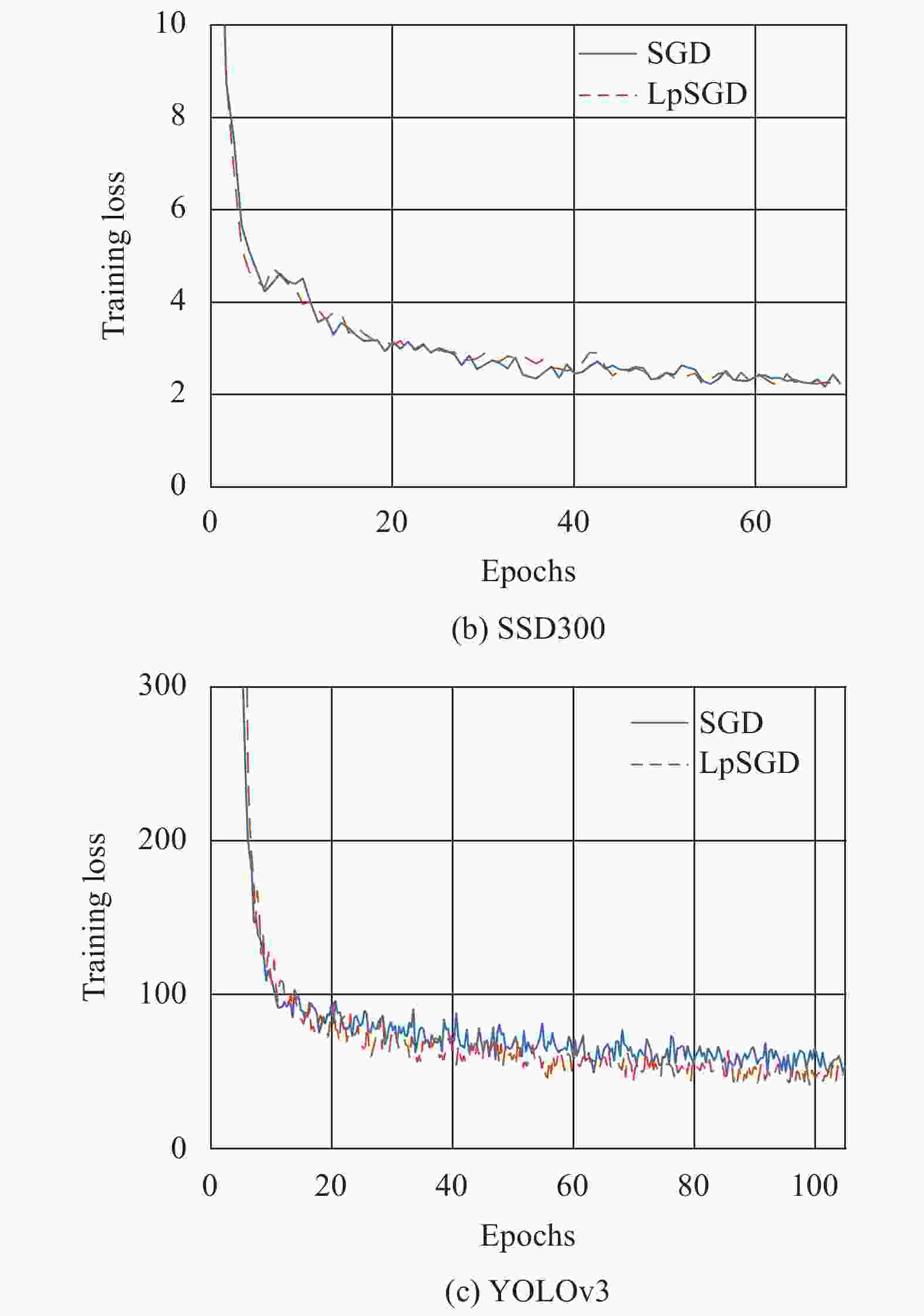
图 5 SGD和LpSGD收敛过程对比
Figure 5. Comparison of convergence process between SGD and LpSGD
-
为更加客观地评价LpSGD,在VOC2007目标检测数据集当中测试稀疏网络相比于稠密网络的参数压缩比例及其准确率变化。为了保证在特征较为丰富的RGB图像当中拥有较高的目标检测准确率,相比于红外目标检测,RGB数据所使用的稀疏网络使用更大的p(p = 1.4)以获得相对较低的稀疏性。各个模型的有效参数的数目和检测精度如表3所示。其中,Faster R-CNN的稀疏模型准确率相比稠密模型降低0.5%,而SSD和YOLOv3的稀疏模型准确率相比稠密模型略微上升0.1%,另一方面SSD和YOLOv3的参数压缩比也显著高于Faster R-CNN,说明在RGB数据集当中,文中的稀疏化方法相比于两阶段模型更加适用于单阶段模型。总体上,相比于红外数据集测试结果,尽管RGB数据集当中稀疏网络的参数压缩比和准确率提升均相对较低,但在显著压缩网络规模的同时依然维持了相当的准确率。一方面展示了文中方法在RGB目标检测网络压缩方面的有效性,另一方面也说明相比于RGB目标检测网络,文中方法更加适用于红外目标检测网络的压缩。
表 3 VOC2007数据集目标检测模型及其结果
Table 3. Object detection model and result on VOC2007 dataset
Method Faster R-CNN SSD 300 YOLOv3 Dense Sparse Dense Sparse Dense Sparse Nonzero parameters Backbone 26 852 416 15 756 216 22 943 936 14 995 952 55 294 688 37 291 638 Detector 14 593 140 14 593 140 3 341 550 3 341 550 6 331 357 6 331 357 AP Aero 0.833 0.826 0.854 0.847 0.801 0.802 Bike 0.781 0.773 0.798 0.795 0.848 0.845 Bird 0.735 0.737 0.702 0.712 0.716 0.726 Boat 0.532 0.528 0.568 0.543 0.652 0.641 Bottle 0.487 0.493 0.457 0.474 0.638 0.647 Bus 0.774 0.765 0.790 0.781 0.861 0.858 Car 0.745 0.748 0.757 0.752 0.858 0.859 Cat 0.887 0.872 0.756 0.765 0.847 0.857 Chair 0.449 0.443 0.871 0.865 0.547 0.541 Cow 0.765 0.771 0.524 0.542 0.715 0.725 Table 0.548 0.536 0.768 0.764 0.690 0.681 Dog 0.865 0.857 0.605 0.612 0.828 0.827 Horse 0.817 0.825 0.868 0.874 0.842 0.846 Mbike 0.804 0.798 0.824 0.846 0.821 0.831 Person 0.794 0.782 0.820 0.811 0.807 0.802 Plant 0.391 0.387 0.458 0.447 0.441 0.437 Sheep 0.723 0.725 0.752 0.747 0.696 0.688 Sofa 0.608 0.595 0.691 0.698 0.699 0.696 Train 0.809 0.814 0.809 0.812 0.825 0.834 Tv 0.612 0.607 0.672 0.667 0.718 0.722 mAP 0.698 0.694 0.717 0.718 0.742 0.743 -
文中提出一种使用Lp归一化权重的红外目标检测网络压缩方法,主要用于改进基于CNN的目标检测架构对红外图像的适应性,在压缩网络规模的同时提升其泛化能力。文中首先阐述了Lp归一化权重的稀疏性可以通过p进行精确控制这一现象,在此基础上提出了文中目标检测网络稀疏化训练的方法。该方法分别使用Lp球面梯度下降与经典梯度下降训练主干网络和检测器,以平衡网络规模与拟合精度。在仿真红外数据集实验当中,其在网络规模和检测精度方面均优于稠密模型:在网络规模上,稀疏化方法将Faster R-CNN、SSD与YOLOv3的有效参数分别减少了52%、78%和66%,大幅压缩了目标检测网络的规模;在检测精度上,稀疏化方法将Faster R-CNN、SSD和YOLOv3的mAP分别提高了0.1%、0.3%和0.2%。在VOC2007数据集实验当中,稀疏化方法将Faster R-CNN、SSD与YOLOv3的有效参数分别减少了27%、30%和29%,且将其mAP分别变化了−0.4%、+0.1%和+0.1%。下面将进一步研究红外图像特征的低秩特性,将Lp归一化与低秩分解相结合,进一步压缩有效参数,提高算法性能。
Infrared object detection network compression using Lp normalized weight
-
摘要: 针对红外图像相比于RGB图像纹理较少的特性,提出一种使用Lp归一化权重的红外目标检测网络压缩方法,旨在改进基于卷积神经网络的目标检测方法对红外图像场景的适应性,在压缩网络规模的同时提升其泛化能力。首先阐述了Lp归一化权重的稀疏性可以通过调节p进行精确控制这一现象。基于该现象,提出了一种目标检测网络稀疏化训练方法。该方法分别使用Lp球面梯度下降与经典梯度下降训练主干网络和检测器,以平衡网络规模与拟合精度。仿真红外数据集测试结果表明,其在网络规模和目标检测精度方面均优于稠密模型:在网络规模上,稀疏化方法将Faster R-CNN、(Single Shot multibox Detector,SSD)与YOLOv3的有效参数分别减少了52%、78%和66%;在检测精度上,稀疏化方法将Faster R-CNN、SSD和YOLOv3的(mean Average Precision, mAP)分别提高了0.1%、0.3%和0.2%,验证了所提出方法的有效性。Abstract: In view of the characteristic that the infrared image has less texture compared with RGB image, an infrared object detection network compression method using Lp normalized weight was proposed. It aimed at improving the adaptability of convolutional neural network based object detection framework to the infrared images, and compressing the scale of network while improving its generalization ability. Firstly, the phenomenon that the sparsity of Lp normalized weight can be precisely controlled by adjusting p was revealed. Based on the phenomenon, a sparsification method for object detection network was proposed. It respectively trained the backbone network and the detector with Lp spherical gradient descent and classical gradient descent, to balance the network scale and fitting accuracy. The tests on simulated infrared image dataset show that, the proposed method is superior to the dense model on both of network scale and detection accuracy: in terms of network scale, the sparsification reduces the effective parameters of Faster R-CNN, Single Shot multibox Detector (SSD) and YOLOv3 by 52%, 78% and 66% respectively; it also improves the mean Average Precision (mAP) of Faster R-CNN, SSD and YOLOv3 by 0.1%, 0.3% and 0.2%, thus verifying the effectiveness of the proposed method.
-
图 2 卷积层权重稀疏性随p的变化
Figure 2. Sparsity of weight with respect to p at convolutional layers
图 3 目标检测网络稀疏化训练流程
Figure 3. Training process of sparse neural network for object detection
图 4 经典网络和稀疏化网络红外目标检测结果对比
Figure 4. Result comparison of infrared object detection between classical neural networks and sparse neural networks
表 1 红外仿真数据集
Table 1. Simulated infrared dataset
Classification Training Test Total Class 1 208 28 236 Class 2 210 26 236 Class 3 219 30 249 Class 4 192 29 221 Total 829 113 942  下载: 导出CSV
表 2 红外仿真数据集目标检测模型及其结果
Table 2. Object detection model and result on simulated infrared dataset
Method Scale AP mAP Backbone Detector Class 1 Class 2 Class 3 Class 4 Faster R-CNN Dense 26 852 416 14 511 140 0.912 0.885 0.927 0.972 0.925 Sparse 5 337 352 14 511 130 0.910 0.875 0.936 0.982 0.926 SSD300 Dense 22 943 936 1 202 958 0.893 0.879 0.914 0.965 0.914 Sparse 4 103 396 1 202 958 0.889 0.867 0.924 0.981 0.917 YOLOv3 Dense 55 294 688 6 245 196 0.914 0.898 0.919 0.972 0.926 Sparse 14 829 742 6 245 196 0.906 0.895 0.927 0.984 0.928
下载: 导出CSV
表 3 VOC2007数据集目标检测模型及其结果
Table 3. Object detection model and result on VOC2007 dataset
Method Faster R-CNN SSD 300 YOLOv3 Dense Sparse Dense Sparse Dense Sparse Nonzero parameters Backbone 26 852 416 15 756 216 22 943 936 14 995 952 55 294 688 37 291 638 Detector 14 593 140 14 593 140 3 341 550 3 341 550 6 331 357 6 331 357 AP Aero 0.833 0.826 0.854 0.847 0.801 0.802 Bike 0.781 0.773 0.798 0.795 0.848 0.845 Bird 0.735 0.737 0.702 0.712 0.716 0.726 Boat 0.532 0.528 0.568 0.543 0.652 0.641 Bottle 0.487 0.493 0.457 0.474 0.638 0.647 Bus 0.774 0.765 0.790 0.781 0.861 0.858 Car 0.745 0.748 0.757 0.752 0.858 0.859 Cat 0.887 0.872 0.756 0.765 0.847 0.857 Chair 0.449 0.443 0.871 0.865 0.547 0.541 Cow 0.765 0.771 0.524 0.542 0.715 0.725 Table 0.548 0.536 0.768 0.764 0.690 0.681 Dog 0.865 0.857 0.605 0.612 0.828 0.827 Horse 0.817 0.825 0.868 0.874 0.842 0.846 Mbike 0.804 0.798 0.824 0.846 0.821 0.831 Person 0.794 0.782 0.820 0.811 0.807 0.802 Plant 0.391 0.387 0.458 0.447 0.441 0.437 Sheep 0.723 0.725 0.752 0.747 0.696 0.688 Sofa 0.608 0.595 0.691 0.698 0.699 0.696 Train 0.809 0.814 0.809 0.812 0.825 0.834 Tv 0.612 0.607 0.672 0.667 0.718 0.722 mAP 0.698 0.694 0.717 0.718 0.742 0.743
下载: 导出CSV
-
[1] Lienhart R, Maydt J. An extended set of Haar-like features for rapid object detection[C]//International Conference on Image Processing, 2002. [2] Dalal N, Triggs B. Histograms of oriented gradients for human detection[C]//IEEE Computer Society Conference on Computer Vision & Pattern Recognition, 2005. [3] Lowe D G. Distinctive image features from scale-invariant keypoints [J]. International Journal of Computer Vision, 2004, 60(2): 91-110. doi: 10.1023/B:VISI.0000029664.99615.94 [4] Bay H, Ess A, Tuytelaars T, et al. Speeded-up robust features [J]. Computer Vision and Image Understanding, 2008, 110(3): 346-359. doi: 10.1016/j.cviu.2007.09.014 [5] Li X, Wang L, Sung E. AdaBoost with SVM-based component classifiers [J]. Engineering Applications of Artificial Intelligence, 2008, 21(5): 785-795. doi: 10.1016/j.engappai.2007.07.001 [6] Felzenszwalb P F, Huttenlocher D P. Pictorial structures for object recognition [J]. International Journal of Computer Vision, 2005, 61(1): 55-79. doi: 10.1023/B:VISI.0000042934.15159.49 [7] Felzenszwalb P F, Girshick R B, McAllester D. Cascade object detection with deformable part models[C]//2010 IEEE Computer Society Conference on Computer Vision and Pattern Recognition, 2010: 2241-2248. [8] Felzenszwalb P F, Girshick R B, Mcallester D A. Visual object detection with deformable part models[C]//The Twenty-Third IEEE Conference on Computer Vision and Pattern Recognition, 2010. [9] Zhang Xiuling, Hou Daibiao, Zhang Chengcheng, et al. Design of MPCANet fire image recognition model for deep learning [J]. Infrared and Laser Engineering, 2018, 47(2): 0203006. (in Chinese) doi: 10.3788/IRLA201847.0203006 [10] Gong Junliang, He Xin, Wei Zhonghui, et al. Infrared dim and small target detection method using scale-space theory [J]. Infrared and Laser Engineering, 2013, 42(9): 2566-2573. (in Chinese) doi: 10.3969/j.issn.1007-2276.2013.09.048 [11] Ren S, He K, Girshick R, et al. Faster R-CNN: Towards real-time object detection with region proposal networks [J]. IEEE Transactions on Pattern Analysis & Machine Intelligence, 2017, 39(6): 1137-1149. [12] Dai J, Li Y, He K, et al. R-FCN: Object detection via region-based fully convolutional networks[C]//Proceedings of the 30th International Conference on Neural Information Processing Systems. 2016: 379-387. [13] Redmon J, Divvala S, Girshick R, et al. You only look once: Unified, real-time object detection[C]//Proceedings of the IEEE Conference on Computer Vision & Pattern Recognition, 2016: 779-788. [14] Liu W, Anguelov D, Erhan D, et al. SSD: Single shot multibox detector[C]//European Conference on Computer Vision, 2016: 21-37. -

 点击查看大图

计量
- 文章访问数: 322
- HTML全文浏览量: 157
- PDF下载量: 36
- 被引次数: 0


