


-
红外成像技术是一项日益成熟的高新技术[1],但是,热红外图空间分辨率较低,容易丢失物体的纹理和轮廓等细节信息;可见光图像的细节信息丰富,但易受拍摄条件影响。红外与可见光图像的融合分析既能克服单源图像的固有缺陷,又能提高信息的冗余性和互补性[2],尤其在智能安防领域,既能监控人的体温,又能判断个体特征差异,有着广阔的应用前景。
图像配准作为图像融合的关键步骤,是寻找图像间的空间变换关系,将图像变换到同一坐标系下的过程。热红外图因为其固有的缺点,特征点检测算法如SIFT、SURF[3]、ORB、HOG[4]、Harris[5]、Kaze[6]等很难提取准确的关键点,所以研究者多在一些电气设备检测上展开此类工作[7],或者利用人像轮廓作为整体特征应用于智能安防[8]。参考文献[9]中是用SURF算法提取特征点,利用斜率一致性筛选配准,准确度高但是算法复杂度高,且普适性差。参考文献[10]对人体轮廓进行了多边形逼近,逼近过程中精度不够,配准结果不理想。参考文献[11]中提出对轮廓进行鲁棒性变换,有效地提高了配准精度,但是不适用于复杂的轮廓处理。参考文献[12]研究了一种基于面部红外成像形成视觉显著图,通过仿射变换,遗传算法优化参数,在对齐人脸后进行有关温度区域依赖性数据分析,但是此法对热像仪成像质量要求较高,对温度精度依赖性很强。
针对现有算法对特征轮廓的应用不足导致精度较差,或是过度处理轮廓导致复杂度高以及普适性差的问题,文中提出一种基于特征轮廓四边形(Featured Contour Quadrilateral, FCQ)的热红外图与可见光图的配准方法。通过对轮廓周长和面积的判断筛选出必要的有核心温度的轮廓,构造出特征轮廓四边形;改进了单应性变换模型,使其具有中和误差的能力,再利用四边形顶点求解单应性变换参数进行配准。FCQ算法可以适用于中近物距(热像仪工作范围内)对人像进行特征轮廓提取和配准,实验验证其高精度的配准效果。
-
热红外图与可见光图的目标轮廓通常存在不小的差异,文中的FCQ算法通过对轮廓筛选并求特征四边形的方式可以避免轮廓差异带来的配准困难,同时也能充分利用轮廓特征保证良好的精度。如图1所示,FCQ配准算法的具体步骤如下:
(1)初始化处理图像,通过Grabcut算法和Mean-Shift算法粗分割图像的前景和背景。
(2)灰度化处理。
(3)特征轮廓的提取,提取轮廓点,重新绘制轮廓并且构建网状结构;再对轮廓进行多边形近似,筛选轮廓,得到2~4个特征轮廓。
(4)生成特征四边形,将步骤(3)中得到的所有轮廓点存入一个点集,求出此点集的外接特征四边形。
(5)求解单应性变换矩阵,将热红外图和可见光图上的四边形顶点代入改进的单应性变换模型,得到矩阵的八个参数值。
(6)配准融合,通过单应性变换对热红外图进行配准,再将已配准图像和可见光图像进行叠加融合。
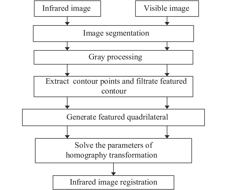
图 1 所提算法的流程图
Figure 1. Flow chart of the proposed algorithm in this paper
-
文中使用Grabcut算法和Mean-Shift算法对图像进行预处理。首先使用Grabcut将人像粗分割出来,再通过滑动窗口寻找同一类型的像素点并统一像素点的像素值,可以输出一个颜色区域边界清晰,细纹纹理更少且平缓的人像图片。
(1) Mean-Shift向量定义
给定d维空间中的n个样本点
${x_i}$ ,其中i=1,…,n,x点的Mean-Shift向量的基本形式为:$${M_h}\left( x \right) \equiv \frac{1}{k}\sum\limits_{{x_i} \in {S_h}} {\left( {{x_i} - x} \right)} $$ (1) 式中:k为在这n个样本点
${x_i}$ 中有k个点落入${S_h}$ 区域中;${S_h}$ 是一个半径为h的高维球区域,是满足以下关系的y点的集合:$${S_h}\left( x \right) \equiv \left\{ {y:{{\left( {y - x} \right)}^{\rm T}}\left( {y - x} \right) \leqslant {h^2}} \right\}$$ (2) (2) 迭代空间构建
以输入图像上任一点
${P_0}$ 为球心,建立物理空间上半径为${S_p}$ ,色彩空间上半径为${C_r}$ 的五维球形空间。文中热红外图与可见光图的${S_p}$ 和${C_r}$ 分别为(20,20)和(1,70),根据不同场景可以调整。在球形空间中,求得所有点相对于中心点的色彩向量之和,移动迭代空间的中心点到该向量的终点,直到在最后一个空间球体中所求得的向量和的终点就是该空间球体的中心点${P_n}$ ,迭代结束。点${P_0}$ 的色彩值为本轮迭代的终点${P_n}$ 的色彩值,如此完成每一个点的色彩均值漂移,初步分割前景和背景。 -
对预处理后的图像使用Canny算子检测边缘,并进行灰度二值化,再对二值图像进行轮廓检索和提取。文中FCQ算法使用轮廓逼近方式进行轮廓点检测,可以减少返回点的数目。
(1) 定义离散曲率
对于曲线
$y = f\left( x \right)$ ,使用曲率检测法[13]给出点${P_i}$ 的离散曲率$S\left( {{P_i}} \right)$ 的定义:$$S\left( {{{{p}}_i}} \right) = {f_{i + 1}} - {f_i}$$ (3) (2) 确定闭曲线上点
${P_i}$ 的支持域任取点
${P_i}$ 前后两点${P_{i - k}}$ 和${P_{i + k}}$ ,$\overline {{P_{i - k}}{P_{i + k}}} $ 为曲线上的一个弦,弦的长度${l_{ik}}$ 为:$${l_{ik}} = \left| {\overline {{P_{i - k}}{P_{i + k}}} } \right|$$ (4) 设
${d_{ik}}$ 为点${P_i}$ 的到弦$\overline {{P_{i - k}}{P_{i + k}}} $ 的垂直距离。从k=1开始,计算${l_{ik}}$ 和${d_{ik}}$ ,判断是否满足以下两个条件1)和2)的任意一个:$$ {{1}})\;\;\;\;\;\;\;\;{l_{ik}} \geqslant {l_{i,k + 1}} $$ (5) $$ {{2}})\;\;\;\;\;\;\;\;\;\frac{{{d_{ik}}}}{{{l_{ik}}}} \geqslant \frac{{{d_{i,k + 1}}}}{{{l_{i,k + 1}}}}\;\;\;{\text{其中}}\;\;\;{d_{ik}}>0 $$ (6) $$ \frac{{{d_{ik}}}}{{{l_{ik}}}} \leqslant \frac{{{d_{i,k + 1}}}}{{{l_{i,k + 1}}}}\;\;\;{\text{其中}}\;\;\;{d_{ik}} <0 $$ (7) k的最大值即是点
${P_i}$ 支持域的半径,记为${k_i}$ ,则${P_i}$ 的支持域是满足条件1)或者2)的点集,即$$D\left( {{P_i}} \right) = \left\{ {\left( {{P_{i - {k_i}}}, \cdot \cdot \cdot ,{P_{i - 1}},{P_i},{P_{i + 1}}, \cdot \cdot \cdot ,{P_{i + {k_i}}}} \right)| 1 )\parallel 2)} \right\}$$ (8) (3) 返回轮廓点
1)使用曲率检测作为显著性度量并计算每个点的曲率绝对值
$\left| {S\left( {{P_i}} \right)} \right|$ 。2)非最大值抑制,保留满足以下条件的点。
$$\left| {S\left( {{P_i}} \right)} \right| \geqslant \left| {S\left( {{P_j}} \right)} \right|$$ (9) 式中:j满足
$\left| {i - j} \right| \leqslant {k_i}/2$ 。3)进一步抑制所有具有0曲率的点。
4)针对3)剩下的点,如果
$D\left( {{P_i}} \right)$ 中的${k_i}$ =1,并且${P_{i - 1}}$ 或${P_{i + 1}}$ 仍然存在,则进一步将满足$\left| {S\left( {{P_i}} \right)} \right| \leqslant $ $ \left| {S\left( {{P_{i - 1}}} \right)} \right|$ 或$\left| {S\left( {{P_i}} \right)} \right| \leqslant \left| {S\left( {{P_{i + 1}}} \right)} \right|$ 的点${P_i}$ 抑制掉。5)对于存活超过两个点的点集
$D\left( {{P_i}} \right)$ ,抑制除点集的两个端点之外的所有点;对于点集中只有两个点的情况:如果$\left| {S\left( {{P_i}} \right)} \right| > \left| {S\left( {{P_{i + 1}}} \right)} \right|$ ,则排除点${P_{i + 1}}$ ,如果$\left| {S\left( {{P_i}} \right)} \right| < \left| {S\left( {{P_{i + 1}}} \right)} \right|$ ,则排除点${P_i}$ 。该算法可以从第一个轮廓点开始顺序处理,步骤2)之后,仍存的点数通常仅是总输入轮廓点的一小部分;步骤3)基本上消除具有零曲率的点,步骤4)需要照顾支持域为1的点。图2为返回点的图示,图2(a)为一个轮廓曲线,图2(b)上红色的点为所返回的轮廓点,可见此方法有效减少了返回点的数目,平滑了曲线,并且可以保留曲线的特征。
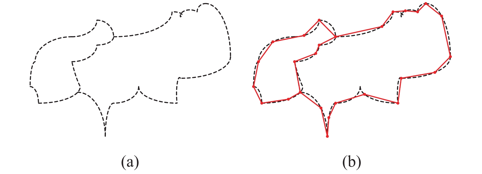
图 2 轮廓特征点的检测
Figure 2. Detection of contour feature points
(4)筛选出特征轮廓
对于热红外图和可见光图,检索出来的轮廓数量和轮廓点都不尽相同,分别提取两图像的轮廓点后对它们进行绘制,再将轮廓进行编号建立网状结构,计算每个轮廓的周长
$l$ 和面积s,得到两个数组:$$L{\rm{ = }}\left[ {{l_1},{l_2} ,\cdot \cdot \cdot ,{l_i}} \right]$$ (10) $$S{\rm{ = }}\left[ {{s_1},{s_2}, \cdot \cdot \cdot ,{s_i}} \right]$$ (11) 式中:
$i$ 为轮廓的个数,$i > 0$ 。设置周长阈值a和面积阈值b,使得周长和面积满足:$$\left( {{l_i} \geqslant a} \right) \cup \left( {{s_i} \geqslant b} \right)$$ (12) 通过公式(12)筛选周长和面积同时为最大的2~4个轮廓,若轮廓数小于2,则迭代降低a,b的值直到轮廓数符合要求;若轮廓数大于4,则调高阈值。这样可以剔除目标人像外部和内部仍存在的干扰轮廓,得到的就是待配准的特征轮廓,再对其进行多边形近似,如图3所示。

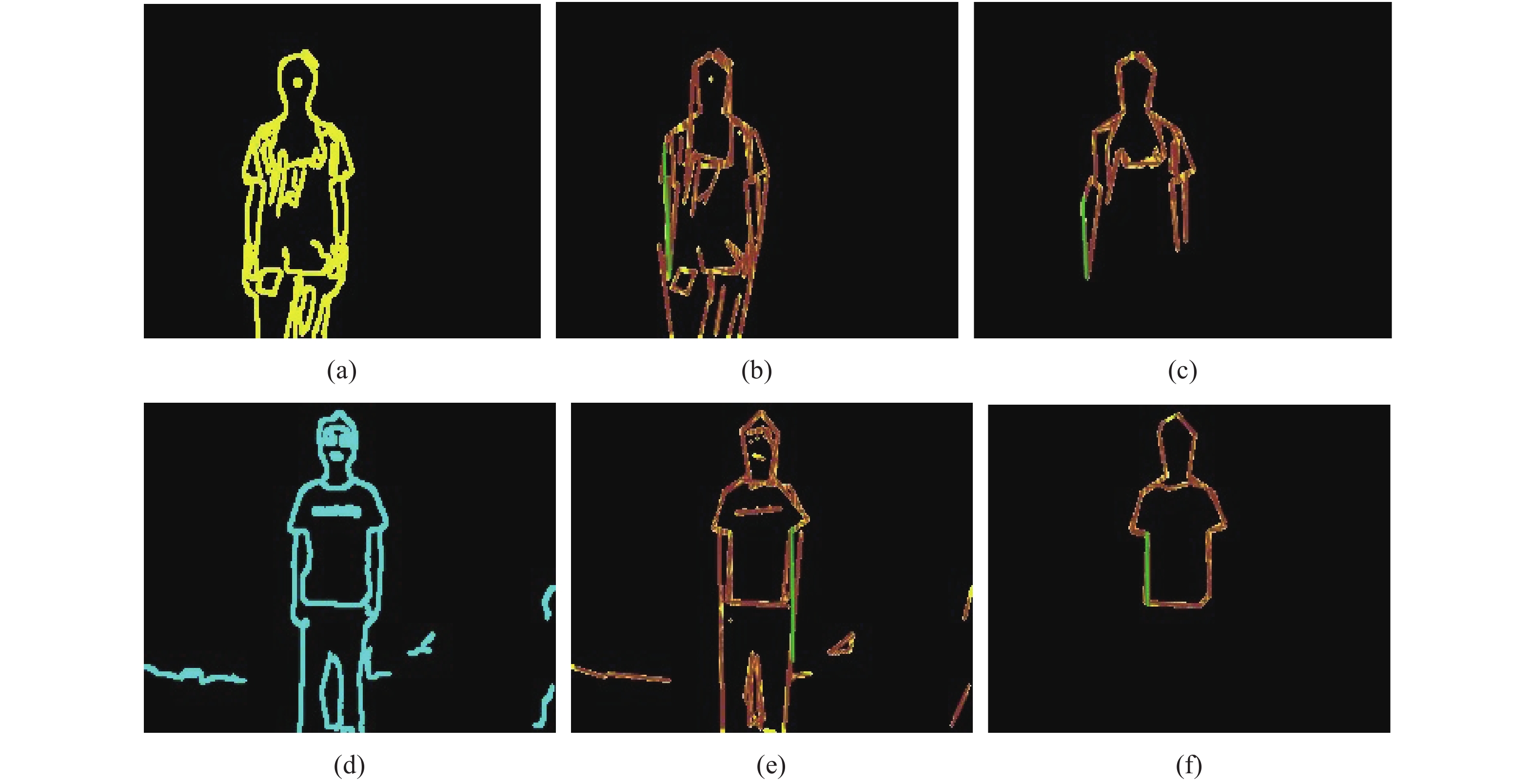
图 3 特征轮廓 。(a)、(d) 传统方式下进行的提取的热红外图和可见光图的轮廓;(b)、(e) 参考文献[10]中对轮廓进行了多边形逼近;(c)、(f) 文中FCQ算法所提取的特征轮廓
Figure 3. Featured contour. (a), (d) Contours of thermal infrared image and visible light image extracted by traditional method; (b), (e) Polygon approximation of contours in reference [10]; (c), (f) Featured contours extracted by proposed FCQ algorithm
从图3可以看到,图3(a)和(d)显示没有减少返回的点数,还会受到目标外部轮廓的干扰。图3(b)和(e)示出得到的特征多边形差异较大。图3(c)和(f)是文中FCQ算法得到的特征轮廓,减少了返回的点数,只保留了可用于配准的轮廓,且消除了一定的干扰,只需要再求其外接四边形就可以进行配准。
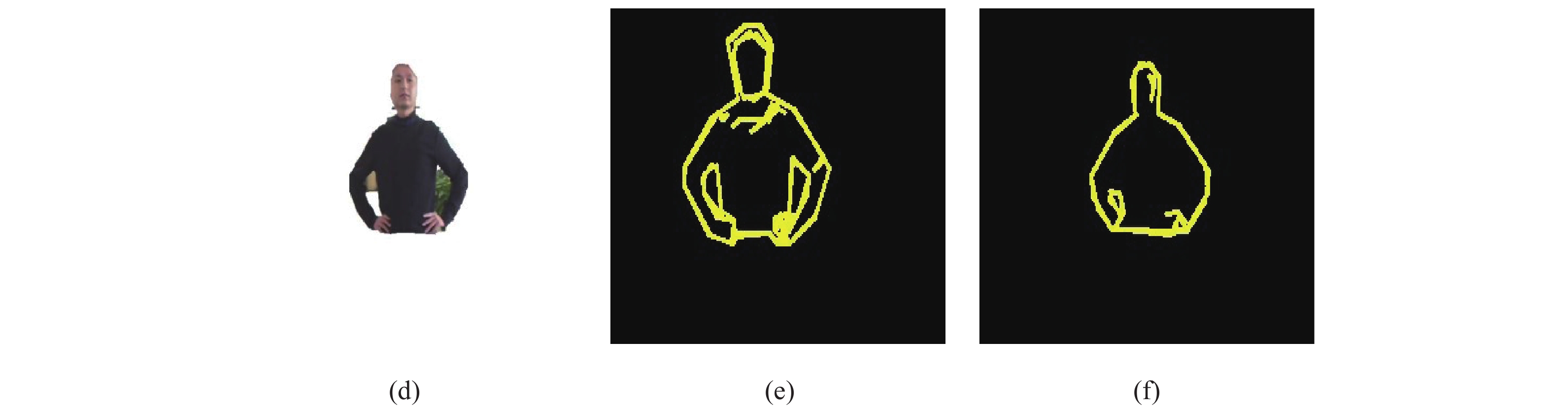
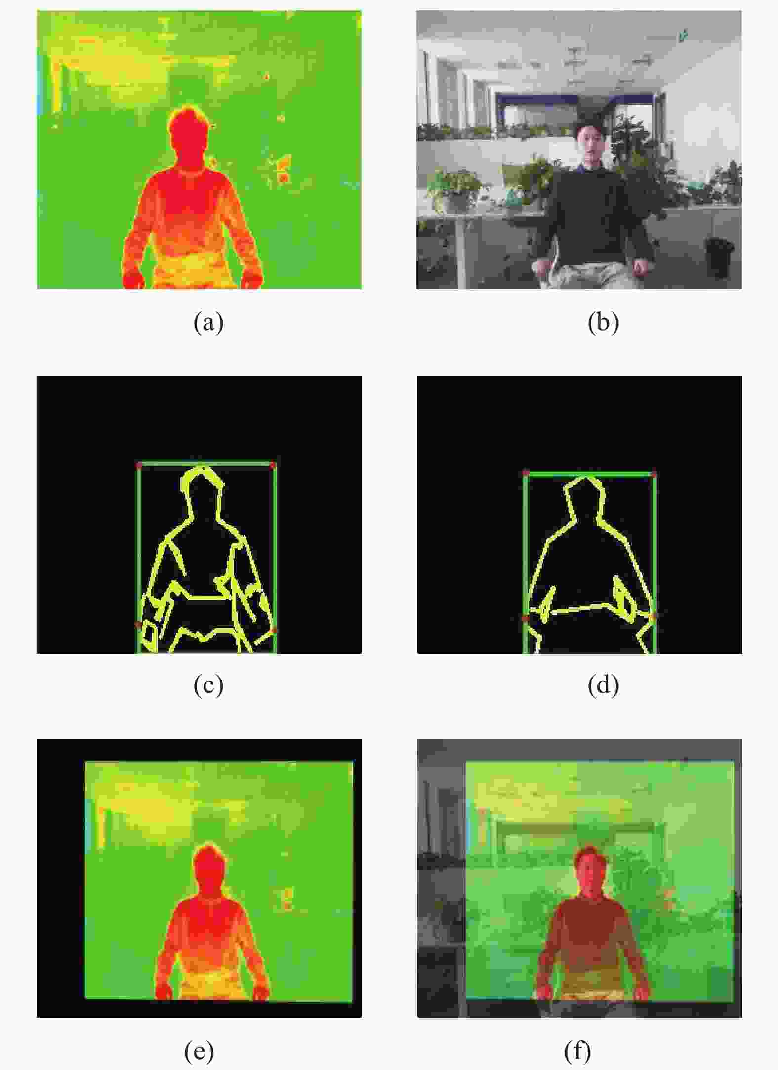
图4是一组复杂背景下提取的特征轮廓,图4(a)和(b)为热红外图和可见光图像,经过人像粗分割后得到图4(c)和(d),图4(e)和(f)为提取到的特征轮廓。
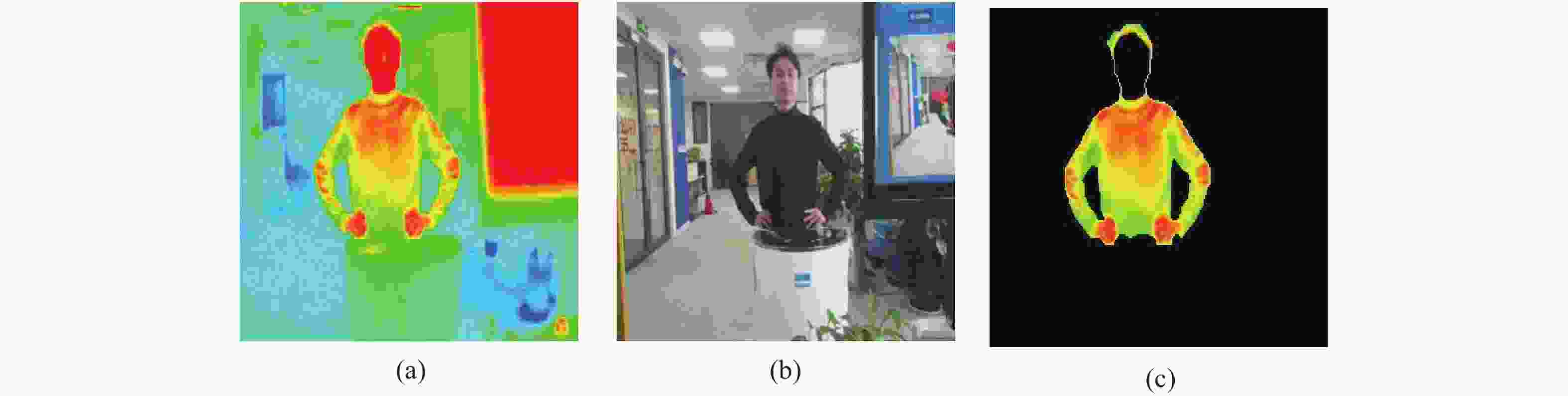
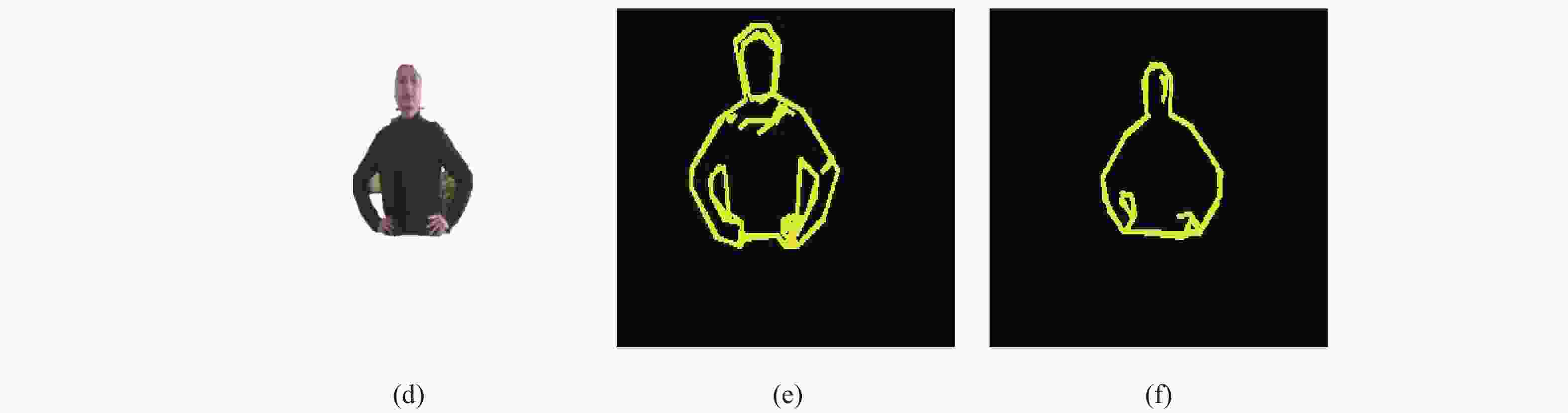
图 4 复杂背景下提取的热红外图和可见光图的特征轮廓
Figure 4. Feature contours of thermal infrared and visible images extracted under complex background
-
将特征轮廓图上的点全部存入一个点集中,生成外接四边形,四边形可能超出图像的边界,此时需要求出四边形与特征轮廓的左交点和右交点,记它们的纵坐标分别为
$\left( {{m_1},{m_2}, \cdots ,{m_n}} \right)$ 和$\left( {{n_1},{n_2}, \cdots ,{n_m}} \right)$ 。对这两组纵坐标分别按大小排序,取其中位数${m_a},{n_b}$ ,则特征四边形的四个顶点就是矩形的两个上顶点和纵坐标为${m_a}$ 的左交点、纵坐标为${n_b}$ 的右交点,输出这四个点进行参数计算。图5为利用第2.2节步骤(4)中筛选的特征轮廓绘制特征四边形的算法过程。

图 5 生成特征轮廓四边形的算法流程图
Figure 5. Algorithm flow chart for generating featured contour quadrilateral
-
实际应用中热像仪与普通镜头的位置、角度和成像焦距不同,不能保证图像的平直行。为了提高配准的可靠性和灵活性,文中采用了单应性变换。
单应性变换具有八个自由度。可以表示为:
$$\left( {\begin{array}{*{20}{c}} {x'} \\ {y'} \\ 1 \end{array}} \right) = \left[ {\begin{array}{*{20}{c}} {{A_{2 \times 2}}}&{{T_{2 \times 1}}} \\ {{V^{\rm T}}}&s \end{array}} \right]\left( {\begin{array}{*{20}{c}} x \\ y \\ 1 \end{array}} \right)$$ (13) 式中:旋转矩阵
${A_{2 \times 2}} = \left[ {\begin{array}{*{20}{c}} {{a_{00}}}&{{a_{01}}} \\ {{a_{10}}}&{{a_{11}}} \end{array}} \right]$ 表示的是仿射变换参数矩阵;${T_{2 \times 1}} = \left[ {\begin{array}{*{20}{c}} {{t_x}} \\ {{t_y}} \end{array}} \right]$ 表示x,y方向上的平移量;${V^{\rm T}} = \left[ {{v_1},{v_2}} \right]$ 表示一种“变换后边缘交点”关系;s是一个与${V^{\rm T}} = \left[ {{v_1},{v_2}} \right]$ 有关的缩放因子。 -
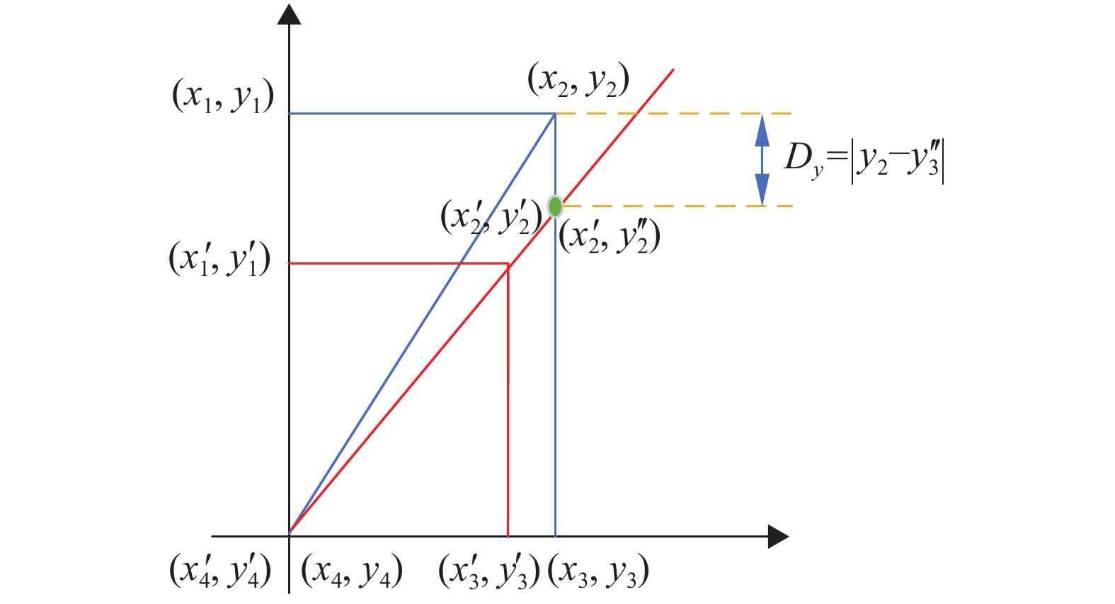
热红外图和可见光图的成像原理不同,求得的两个特征轮廓不能完全契合,为了消除误差,需要优化单应性变换模型。假定热红外图的特征四边形顶点为
$\left( {{x_1},{y_1}} \right)$ ,$\left( {{x_2},{y_2}} \right)$ ,$\left( {{x_3},{y_3}} \right),\left( {{x_4},{y_4}} \right)$ ,可见光图的特征四边形顶点为$\left( {{{x'}_1},{{y'}_1}} \right),\left( {{{x'}_2},{{y'}_2}} \right),\left( {{{x'}_3},{{y'}_3}} \right),\left( {{{x'}_4},{{y'}_4}} \right)$ ,优化的单应性变换参数计算步骤如下:(1)分别计算两个四边形的对角线的斜率
$k$ 和$k'$ :$$k = \left| {\frac{{{y_2} - {y_4}}}{{{x_2} - {x_4}}}} \right|$$ (14) $$k' = \left| {\frac{{{{y'}_2} - {{y'}_4}}}{{{{x'}_2} - {{x'}_4}}}} \right|$$ (15) 则设置修正后的斜率
$k''$ 为:$$k'' = \min \left( {k,k'} \right)$$ (16) (2)以可见光图特征四边形的点
$\left( {{{x'}_4},{{y'}_4}} \right)$ 为起点,画一条直线L:$$L:y - {y'_4} = k''\left( {x - {{x'}_4}} \right)$$ (17) (3)代入
$x = {x'_2}$ ,得到$y = {y''_2}$ 。设立一个位移变量偏差值${D_y}$ ,使得:$${D_y} = \left| {{y_2} - {{y''}_2}} \right|$$ (18) 图6为位移变量偏差值的计算。
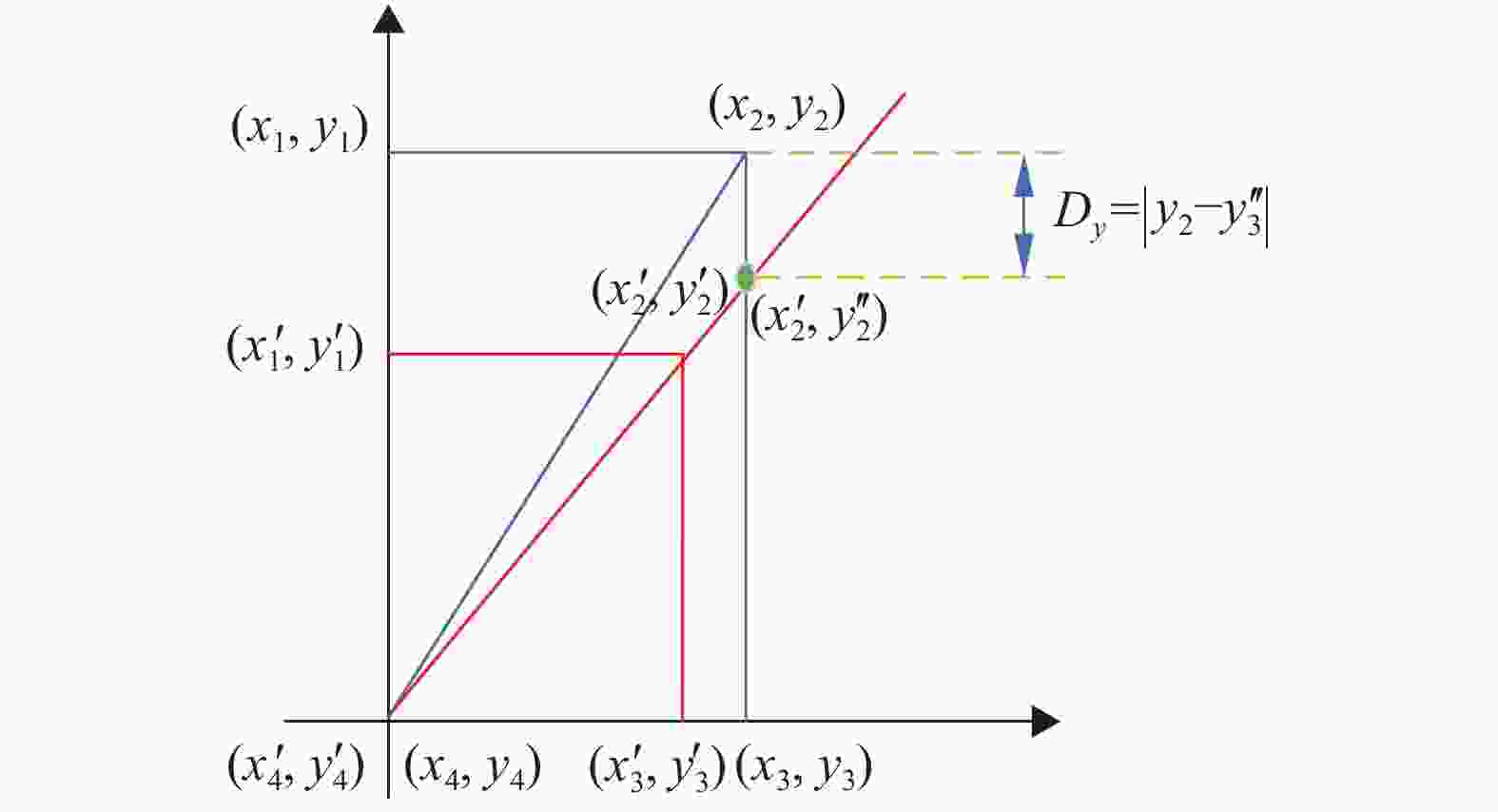
图 6 位移变量偏差值的计算
Figure 6. Calculation of displacement variable deviation value
(4)对变换矩阵中的位移变量进行调整,点
$\left( {{x_2},{y_2}} \right)$ 对应的改进的单应性变换(Improved Homography Transformation, IHT )过程如下:$$\left( {\begin{array}{*{20}{c}} {{{x'}_2}} \\ {{{y'}_2}} \\ 1 \end{array}} \right) = \left[ {\begin{array}{*{20}{c}} {{a_{00}}}&{{a_{01}}}&{{t_x}} \\ {{a_{10}}}&{{a_{11}}}&{{t_y} - {D_y}} \\ {{v_1}}&{{v_2}}&s \end{array}} \right]\left( {\begin{array}{*{20}{c}} {{x_2}} \\ {{y_2}} \\ 1 \end{array}} \right)$$ (19) 实际上,当旋转角度足够小时,可直接在单应性矩阵求解过程中对指定顶点坐标进行调整:
$$\left( {\begin{array}{*{20}{c}} {{{x'}_2}} \\ {{{y'}_2}} \\ 1 \end{array}} \right) = \left[ {\begin{array}{*{20}{c}} {{a_{00}}}&{{a_{01}}}&{{t_x}} \\ {{a_{10}}}&{{a_{11}}}&{{t_y}} \\ {{v_1}}&{{v_2}}&s \end{array}} \right]\left( {\begin{array}{*{20}{c}} {{x_2}} \\ {{y_2} - {D_y}} \\ 1 \end{array}} \right)$$ (20) (5)同理,根据场景也可以设置
${t_x}$ 。针对该点可以列出变换函数:$$\begin{array}{l} \left[ {\begin{array}{*{20}{c}} {{a_{00}}}&{{a_{01}}}&{{t_x} - {D_x}} \\ {{a_{10}}}&{{a_{11}}}&{{t_y} - {D_y}} \\ {{v_1}}&{{v_2}}&s \end{array}} \right]\left( {\begin{array}{*{20}{c}} {{x_2}} \\ {{y_2}} \\ 1 \end{array}} \right) = \left( {\begin{array}{*{20}{c}} {{a_{00}}x + {a_{01}}{y_2} + {t_x} - {D_x}} \\ {{a_{10}}x + {a_{11}}{y_2} + {t_y} - {D_y}} \\ {{v_1}{x_2} + {v_2}{y_2} + s} \end{array}} \right) \Leftrightarrow \\ \left( {\begin{array}{*{20}{c}} {\dfrac{{{a_{00}}{x_2} + {a_{01}}{y_2} + {t_x} - {D_x}}}{{{v_1}x + {v_2}{y_2} + s}}} \\ {\dfrac{{{a_{10}}{x_2} + {a_{11}}{y_2} + {t_y} - {D_y}}}{{{v_1}{x_2} + {v_2}{y_2} + s}}} \end{array}} \right) \end{array}$$ (21) 这里使用归一化使s=1。所以变换矩阵有八个未知数,一组匹配点从
$\left( {{x_i},{y_i}} \right)$ 到$\left( {{{x'}_i},{{y'}_i}} \right)$ 对应有两个方程,只需要四组不共线的匹配点即可求出变换矩阵。 -
文中实验环境的配置为英特尔Core i5-8265U @ 1.60 GHz四核,8 G内存,开发平台为Visual Studio 2019和Opencv3.4.3。模拟在安检等体温检测的实际需求环境下,使用热像仪和普通摄像头,距离目标0.5~3 m,热像仪的焦距短于普通摄像头。所获得的热红外图分辨率为256×196,可见光图分辨率639×480,将可见光图缩小至热红外图大小。使用SURF检测算法提取特征点,筛选最优匹配特征点进行配准,得到的图像作为对照组进行分析。
-
实验一,相对于目标在同一视角下,目标距离两个传感器2 m,两个传感器的轴线平行,因为在远距离的复杂背景下配准难度大,下面先给出两对简单环境下的实例。
(1)第一组单人配准结果
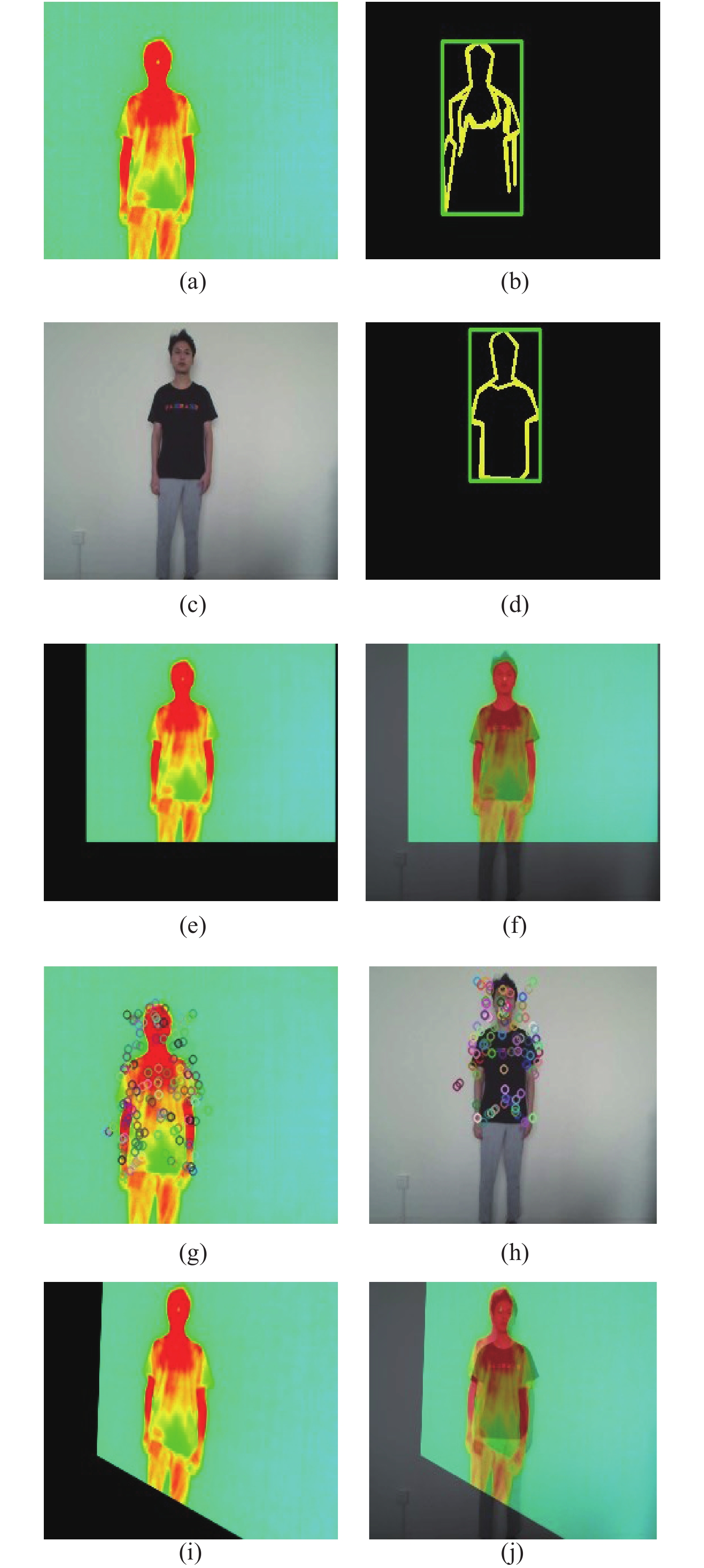
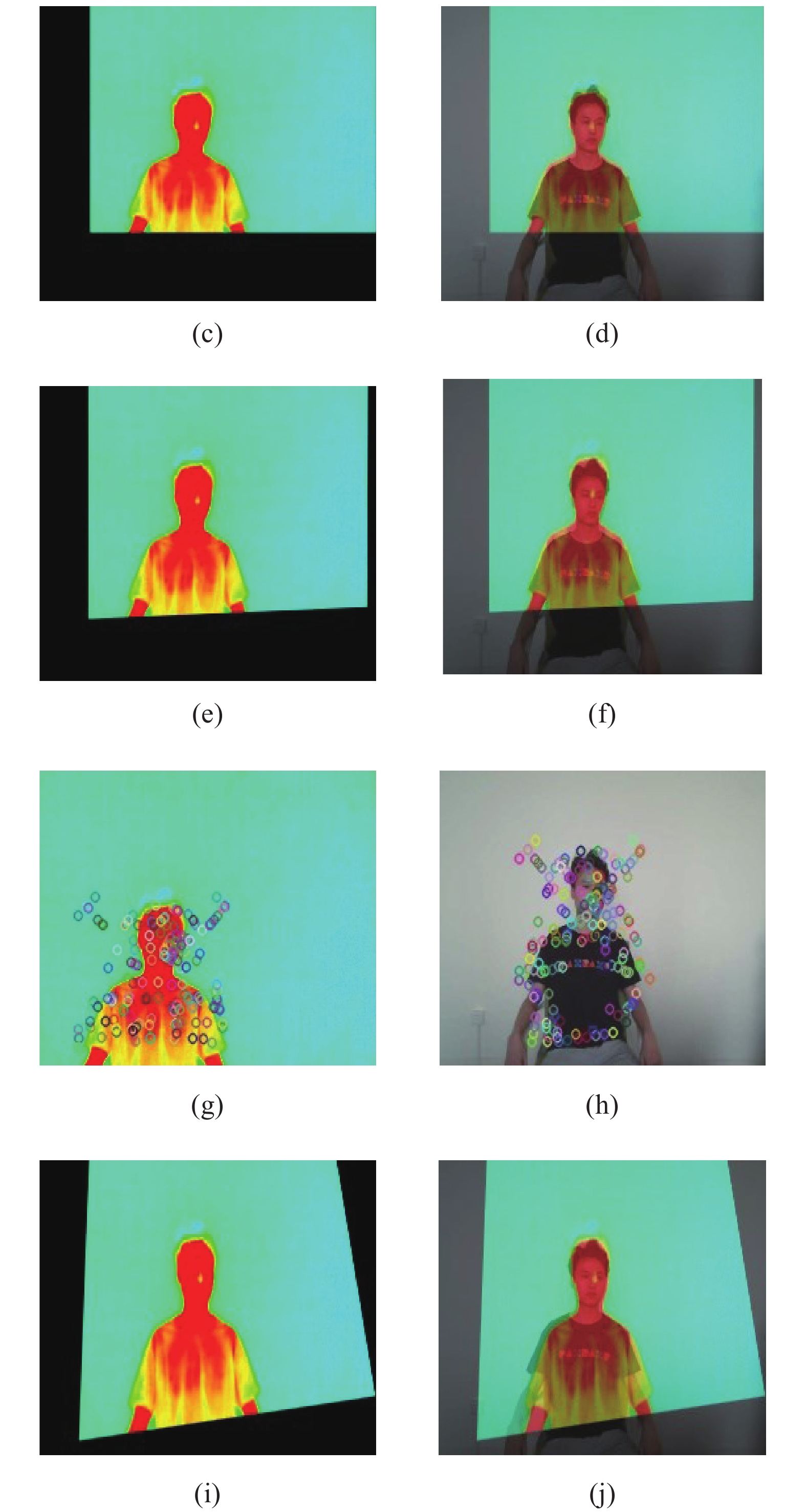
图7为单人图像配准结果图,其中图7(a)和(c)为待配准的热红外图与可见光图,图7(b)和(d)为FCQ算法得到的特征轮廓四边形,筛选出的特征轮廓虽有差异,但外接四边形可避免这种差异对配准的影响。图7(e)为图7(a)经过改进的单应性变换得到的图,图7(f)为配准后的融合图,在视觉上几乎可以做到人像完全重合。在对照组中图7(g)和(h)分别为使用SURF检测算法提取特征点的热红外图和可见光图像,图7(i)为使用SURF特征点配准后的图像,图7(j)为融合图像,可以看到配准结果很不理想。

图 7 实验一第一组热红外图和可见光图配准结果
Figure 7. The first registration result of thermal infrared image and visible image in experiment 1
(2)第二组多人配准结果
图8为第二组多人配准结果,图像中内容多,获得的轮廓数量增加,此时适当调整图像分割参数
${S_p}$ 和${C_r}$ ,减小轮廓过滤时的阈值,以获得更多的特征轮廓。此时外接矩形的下边超出了图像的下边界,使用矩形左右两边上的轮廓点代替,输出四个点为图8(b)、(d)上的红色标点。图8(e)为图8(a)进行改进的单应性变换(IHT)得到的图,图8(f)为多人配准后的融合结果,重合度很高。图8(g)和(h)示出由于使用传统的单应性变换导致肉眼可见的偏差。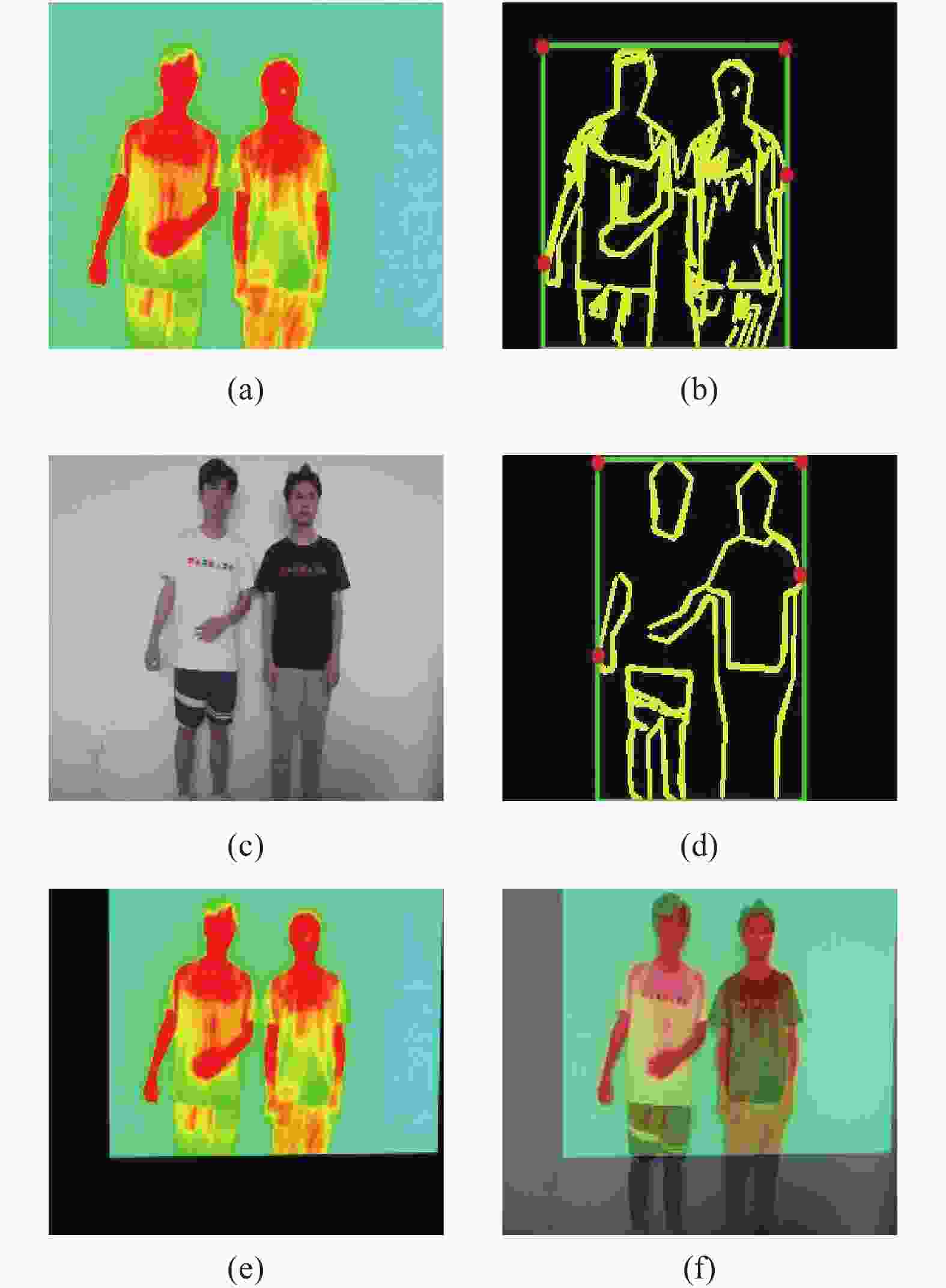
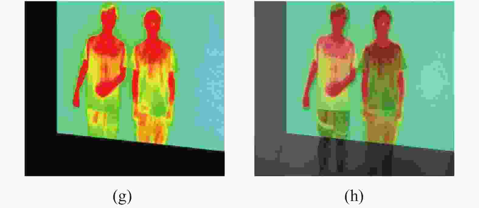
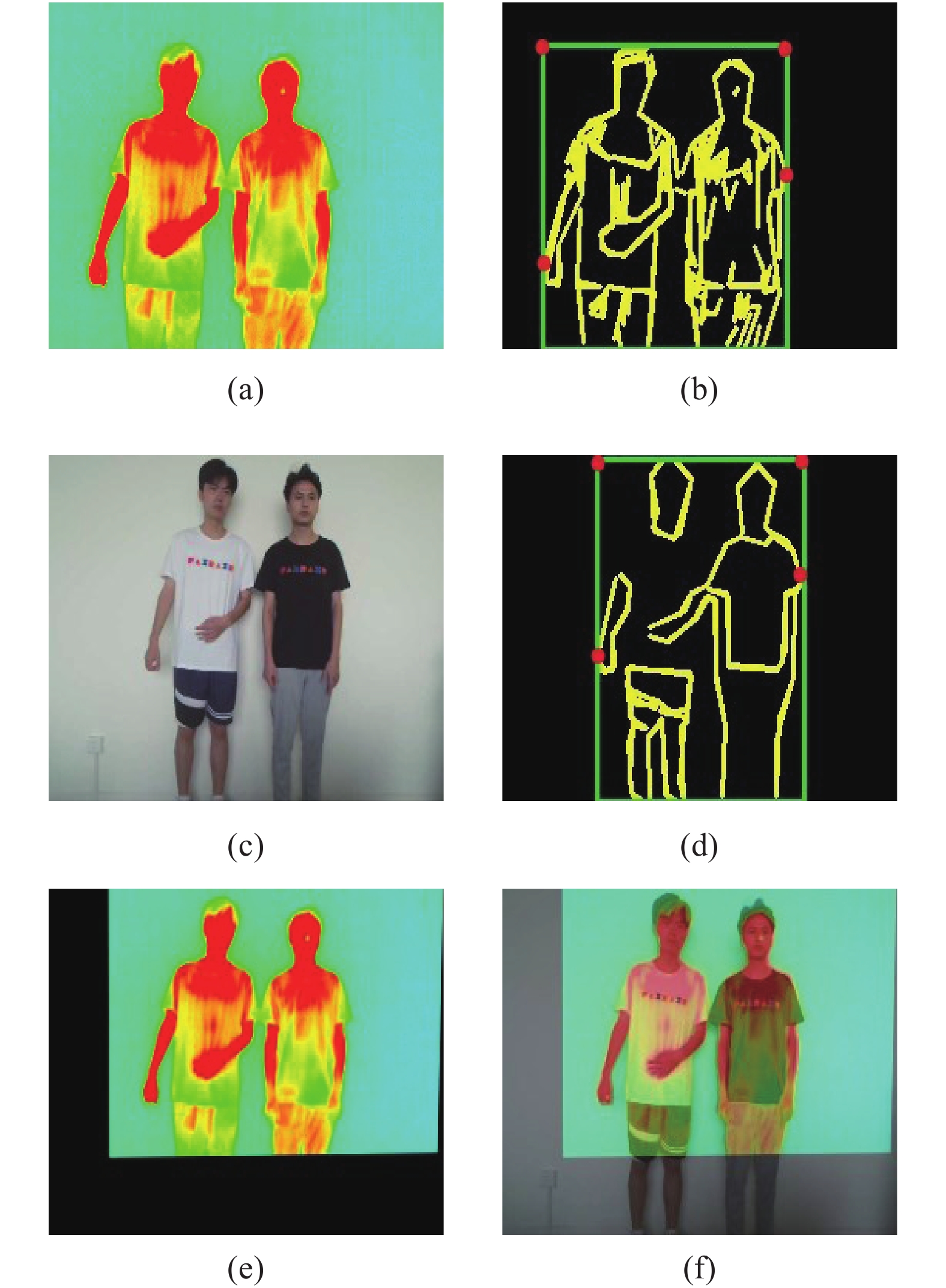
图 8 实验一第二组热红外图和可见光图配准结果。(a)、(b) 热红外图和它的特征轮廓四边形;(c)、(d)可见光图和它的特征轮廓四边形;(e)、(f) FCQ算法应用了改进单应性变换的配准图和融合图;(g)、(h) FCQ算法应用传统单应性变换的配准图和融合图
Figure 8. The second group of thermal infrared image and visible image registration results in experiment 1. (a), (b) Thermal infrared image and its featured contour quadrilateral; (c), (d) Visible image and its featured contour quadrilateral; (e), (f) Registration graph and fusion graph of the FCQ algorithm using improved homography transformation; (g), (h) Registration graph and the fusion graph of FCQ algorithm applying traditional homography transformation
-
实验二,相对于目标在同一视角下,改变实验一中两个传感器的相对位置,物距缩小至1.5 m。在当前距离下,图像中周长最长,面积最大的轮廓是人体的躯干部分,其他对配准作用不大或造成干扰的轮廓被滤除,并且人体的核心温度也集中在头部和躯干部分,所以只保留躯干部分以上,对后面的温度检测也十分有利。加入复杂背景的样本进行研究,下面给出实验结果。
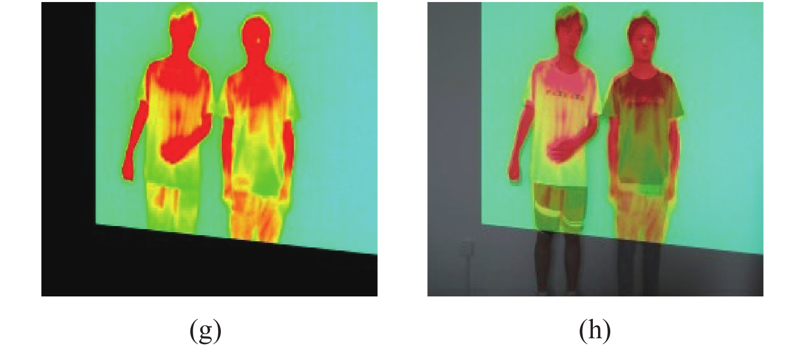
图9为实验二的融合结果。热红外图(图9(a))和可见光图(图9(b))存在背景干扰,图9(c)和(d)分别为图9(a)和图9(b)的特征轮廓四边形图,图9(e)和图9(f)为配准后融合的结果,图9(g)和(h)则是没有应用改进的单应性变换得到的结果,有明显可见的误差。但是在物距变小的情况下,该误差还是要小于实验一中的。FCQ算法可以在背景干扰下实现准确的配准融合,而使用SURF检测得到的对照组图像图9(i)~(l)图像,配准精度仍然不够理想。
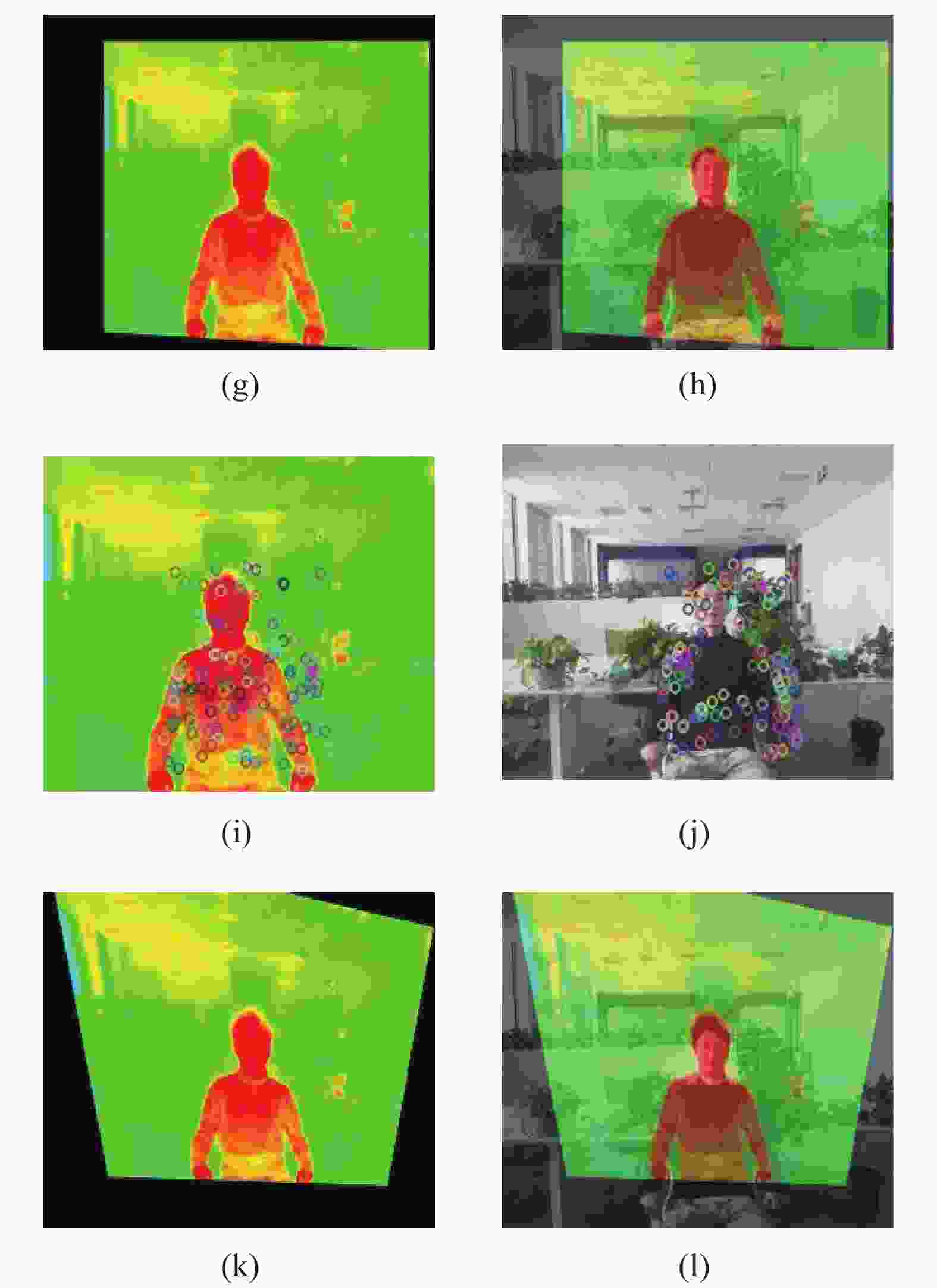
图 9 实验二热红外图和可见光图配准结果
Figure 9. Registration results of thermal infrared image and visible image in experiment 2
-
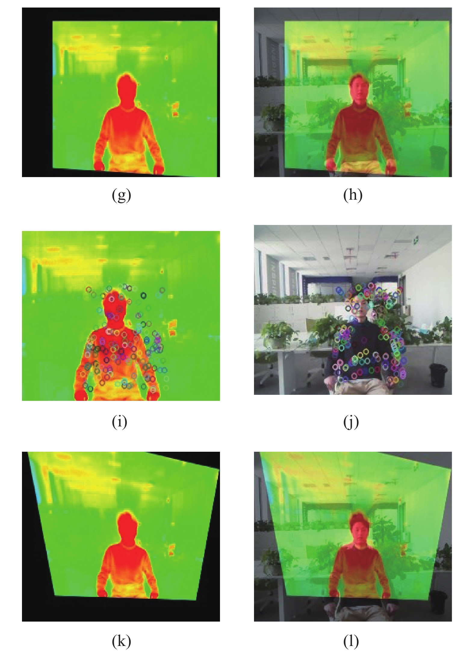
实验三,目标仍然在同一视角下,当目标距离两个传感器0.8 m时,传感器间相对位置不变,传感器轴线依然平行。如图10(a)、(b)所示,过近的物距下图像中目标人像的内容更少,且热图像与可见光图像中的人像内容差距也更大,因此图10(d)中配准误差略大,但基本也可做到完全重合。

图 10 实验三热红外图和可见光图配准结果。(a)热红外图;(b)可见光图;(c)配准图;(d)融合图;(e)、(f)没有应用改进的单应性变换得到的结果
Figure 10. Registration result of thermal infrared image and visible image in experiment 3. (a) Thermal infrared image; (b) Visible image; (c) Registration image; (d) Fusion image; (e),(f) Registration graph and the fusion graph without applying the IHT
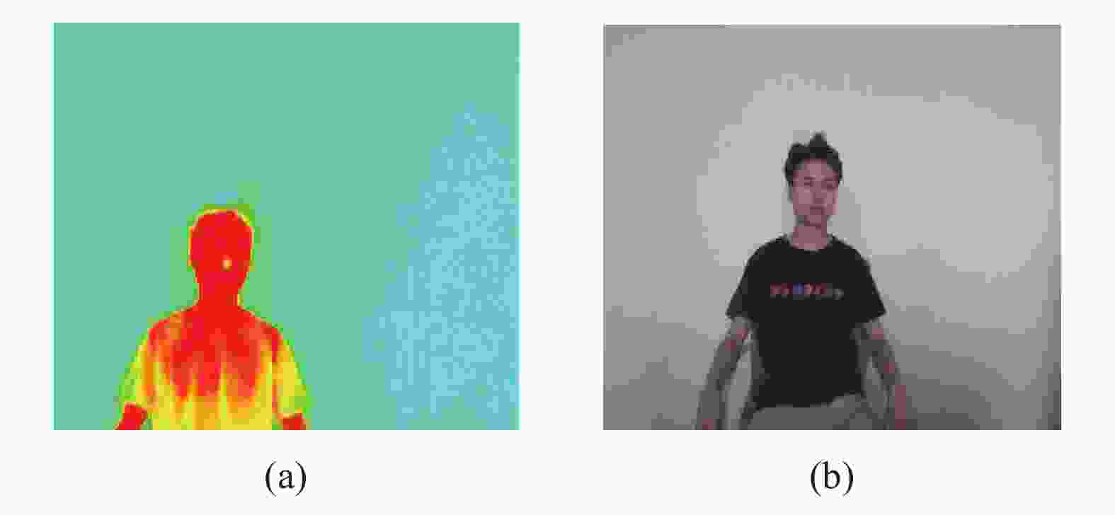
图10(g)~(j)为SURF对照组的实验结果,在平移量、缩放量等配准参数上都存在明显的偏差,配准效果不佳。
-
从图像中随机选取了20对点进行评估,采用均方根误差(RMSE)分析配准精度:
$${\rm{RMSE}} = \sqrt {\dfrac{{ \displaystyle\sum\limits_{i = 1}^{Num} {\left( {errorx_i^2 + errory_i^2} \right)} }}{{Num}}} $$ (22) 其中
$$error{x_i} = {x_i} \cdot s \cdot {a_{00}} + {y_i} \cdot s \cdot {a_{01}} + {t_x} - {x'_i}$$ (23) $$error{y_i} = - {x_i} \cdot s \cdot {a_{10}} + {y_i} \cdot s \cdot {a_{11}} + {t_y} - {y'_i}$$ (24) 式中:Num为选取点对的数目;
${a_{00}},{a_{01}},{a_{10}},{a_{11}},s,{t_x},{t_y}$ 均为配准参数。使用FCQ算法对三组数据进行实验,计算出单应性变换矩阵的八个参数,表1列举了主要参数。
表 1 实验中的配准矩阵参数
Table 1. Registration matrix parameters in experiments
${a_{00}}$ ${a_{11}}$ ${t_x}$ ${t_y}$ Experiment 1 0.884 0.827 31.652 -10.976 Experiment 2 0.805 6 0.894 1 38.047 13.425 Experiment 3 0.849 0.878 38.283 -21.244 分别计算文中FCQ算法和对比组SURF检测算法在上述实验中配准的MSE、RMSE值,同时引用参考文献[10]、[12]算法中的数据整理如表2所示。
表 2 三组实验以及对比组的MSE, RMSE
Table 2. MSE, RMSE of the three experiments and the comparison groups
Algorithms MSE RMSE SURF- experiment 1 6.033 3 FCQ-experiment 1 without IHT 3.073 7 FCQ-experiment 1 with IHT 1.520 3 1.233 0 SURF-experiment 2 9.273 6 FCQ-experiment 2 without IHT 2.240 0 FCQ-experiment 2 with IHT 1.144 4 1.069 8 SURF-Experiment 3 9.445 6 FCQ-experiment 3 without IHT 2.107 2 FCQ-experiment 3 with IHT 1.593 5 1.262 0 Ref. [10] 6.838 2 2.615 0 Ref. [12] 2.459 4 1.568 2 表2中对应用于SURF算法配准的对照组,误差动辄在10 pixel单元以上,均方根误差也远大于FCQ算法的,在此类异源图像配准过程中,特征点检测算法如SURF等的配准精度很难达到工程应用级别。FCQ算法进行配准实验时的均方根误差都控制在合理的范围内。FCQ算法在使用传统单应性变换时的均方根误差比较大,在物距由远到近变化时,位移变量偏移值越来越小,均方根误差也会越来越小。但在应用了文中的IHT后,在各个物距下的误差都大幅减小,精确度提升了一倍以上。相对而言,物距为0.8 m时的配准内容差异大,配准误差稍大,所以对两个传感器的位置要求更加苛刻。算法运行的最佳物距是1.5 m。
-
FCQ有良好的可靠性和抗干扰性,对于不同场景、不同角度、不同物距(热像仪有效范围内)、不同目标内容,都可实现高精度配准。
在新冠疫情的严峻形势下,在人流量大的场所进行人体快速温度监控有着很大的应用前景。文中提出了一种基于特征轮廓四边形的热红外图和可见光图配准方法,有助于快速地捕获目标的体温和实际轮廓特征,不易受到异源图像特征差异的影响,对于后续的信息融合和风险定位提供了有利条件。文中算法具有良好的可靠性、适用性、稳定性,无需复杂的迭代运算,运行速度快。今后的研究重点是改进特征检测算法以适应异源图像配准,或是应用更为先进的人像分割算法,在更长的物距和更复杂的环境中进行目标人体的快速配准,保证误差在视觉接受范围内,并尽可能减少图像失真。
Registration of thermal infrared image and visible image based on featured contour quadrilateral
-
摘要: 热红外图与可见光图的融合分析在智能安防和故障检测中应用广泛。针对同一场景下两图像在融合过程中难以匹配的问题,提出了一种基于特征轮廓四边形的图像配准方法。首先通过分割算法分别对热红外图和可见光图进行过滤;再进行边缘轮廓点的检测和轮廓的重新绘制;然后通过算法筛选出特征轮廓并进行多边形近似,生成特征轮廓的外接四边形;将此四边形顶点代入改进的单应性变换模型计算参数,其中加入了位移变量偏差值可中和80%的误差;最后,通过单应性变换模型对热红外图进行变换配准。实验结果表明,该方法使轮廓定位更加精确,有效减少了匹配误差,能够实现图像的高精度快速配准。Abstract: The fusion analysis of thermal infrared image and visible image is widely used in intelligent security and fault detection. To solve the problem that it is difficult to match two images in the fusion process in the same scene, an image registration method based on featured contour quadrilateral was proposed. Firstly, the thermal infrared image and the visible image were filtered separately by segmentation algorithm. Secondly, the contour points were detected and the contour was redrawn. Then the featured contour was filtered out by the algorithm and the polygon was approximated, and the minimum circumscribed quadrilateral of all contours was generated. The vertexes of this quadrilateral was substituted to calculate the improved homography transformation parameters, and the deviation value of displacement variable was added to neutralize the error of 80%. Finally, the thermal infrared image was registered through the homography transformation model. The experimental results show that this method effectively reduces the matching error, makes the contour positioning more accurate, and can achieve high-precision and rapid image registration.
-
图 3 特征轮廓 。(a)、(d) 传统方式下进行的提取的热红外图和可见光图的轮廓;(b)、(e) 参考文献[10]中对轮廓进行了多边形逼近;(c)、(f) 文中FCQ算法所提取的特征轮廓
Figure 3. Featured contour. (a), (d) Contours of thermal infrared image and visible light image extracted by traditional method; (b), (e) Polygon approximation of contours in reference [10]; (c), (f) Featured contours extracted by proposed FCQ algorithm
图 4 复杂背景下提取的热红外图和可见光图的特征轮廓
Figure 4. Feature contours of thermal infrared and visible images extracted under complex background
图 5 生成特征轮廓四边形的算法流程图
Figure 5. Algorithm flow chart for generating featured contour quadrilateral
图 7 实验一第一组热红外图和可见光图配准结果
Figure 7. The first registration result of thermal infrared image and visible image in experiment 1
图 8 实验一第二组热红外图和可见光图配准结果。(a)、(b) 热红外图和它的特征轮廓四边形;(c)、(d)可见光图和它的特征轮廓四边形;(e)、(f) FCQ算法应用了改进单应性变换的配准图和融合图;(g)、(h) FCQ算法应用传统单应性变换的配准图和融合图
Figure 8. The second group of thermal infrared image and visible image registration results in experiment 1. (a), (b) Thermal infrared image and its featured contour quadrilateral; (c), (d) Visible image and its featured contour quadrilateral; (e), (f) Registration graph and fusion graph of the FCQ algorithm using improved homography transformation; (g), (h) Registration graph and the fusion graph of FCQ algorithm applying traditional homography transformation
图 9 实验二热红外图和可见光图配准结果
Figure 9. Registration results of thermal infrared image and visible image in experiment 2
图 10 实验三热红外图和可见光图配准结果。(a)热红外图;(b)可见光图;(c)配准图;(d)融合图;(e)、(f)没有应用改进的单应性变换得到的结果
Figure 10. Registration result of thermal infrared image and visible image in experiment 3. (a) Thermal infrared image; (b) Visible image; (c) Registration image; (d) Fusion image; (e),(f) Registration graph and the fusion graph without applying the IHT
表 1 实验中的配准矩阵参数
Table 1. Registration matrix parameters in experiments
${a_{00}}$ ${a_{11}}$ ${t_x}$ ${t_y}$ Experiment 1 0.884 0.827 31.652 -10.976 Experiment 2 0.805 6 0.894 1 38.047 13.425 Experiment 3 0.849 0.878 38.283 -21.244  下载: 导出CSV
表 2 三组实验以及对比组的MSE, RMSE
Table 2. MSE, RMSE of the three experiments and the comparison groups
Algorithms MSE RMSE SURF- experiment 1 6.033 3 FCQ-experiment 1 without IHT 3.073 7 FCQ-experiment 1 with IHT 1.520 3 1.233 0 SURF-experiment 2 9.273 6 FCQ-experiment 2 without IHT 2.240 0 FCQ-experiment 2 with IHT 1.144 4 1.069 8 SURF-Experiment 3 9.445 6 FCQ-experiment 3 without IHT 2.107 2 FCQ-experiment 3 with IHT 1.593 5 1.262 0 Ref. [10] 6.838 2 2.615 0 Ref. [12] 2.459 4 1.568 2
下载: 导出CSV
-
[1] Lv B L, Tong S F, Xu W, et al. Non-uniformity correction of airborne infrared detection system based on inter-frame registration [J]. Chinese Optics, 2020, 13(5): 1124-1137. (in Chinese) doi: 10.37188/CO.2020-0109 [2] Shi Guojun. Target recognition method of infrared imagery via joint representation of deep features [J]. Infrared and Laser Engineering, 2021, 50(3): 20200399. (in Chinese) doi: 10.3788/IRLA20200399 [3] Liu X N, Di H Z, Yang W, et al. Mosaic of cultural relics fragments based on SURF extraction descriptor and Jacquard distance [J]. Optics and Precision Engineering, 2020, 28(4): 963-972. (in Chinese) [4] Wei H, Zhang K, Zheng L, et al. Infrared image target detection of power inspection based on HOG-RCNN [J]. Infrared and Laser Engineering, 2020, 49(S2): 20200411. (in Chinese) [5] Liu X, Chen S, Zhuo, L, et al. Multi-sensor image registration by combining local self-similarity matching and mutual information [J]. Frontiers of Earth Science, 2018, 12: 779-790. [6] Bao W X, Sang Sier, Shen X F. Remote sensing image registration algorithm based on information entropy constraint and KAZE feature extraction [J]. Optics and Precision Engineering, 2020, 28(8): 1810-1819. (in Chinese) doi: 10.3788/OPE.20202808.1810 [7] Dai J D, Chen Y H, Liu Y D, et al. Registration method of infrared and visible images of electrical equipment based on characteristic quadrilateral [J]. Electrical Automation, 2018, 40(6): 112-115. (in Chinese) [8] Yuan H Q, Li Y, W J Y, et al. High precision detection technology of pedestrian face temperature based on infrared thermal image [J]. Infrared Technology, 2019, 41(12): 1181-1186. (in Chinese) [9] Xu J X, Li Q W, Ma Y P, et al. Infrared and visible image registration method for electrical equipment based on slope consistency [J]. Journal of Optoelectronics·Laser, 2017, 28(7): 794-802. (in Chinese) [10] Chakravorty Tanushri, Guillaume-Alexandre Bilodeau, Granger Eric. Automatic image registration in infrared-visible videos using polygon vertices [J]. arXiv, 2014: 1403.4232. [11] Tian T, Mei X G, Yu Y, et al. Automatic visible and infrared face registration based on silhouette matching and robust transformation estimation [J]. Infrared Physics & Technology, 2015, 69: 145-154. [12] Jian B L, Chen C L, Lin C J, et al. Optimization method of IR thermography facial image registration [J]. IEEE Access, 2019, 7: 93501-93510. doi: 10.1109/ACCESS.2019.2927747 [13] Teh C H, Chin R T. On the detection of dominant points on digital curves [J]. IEEE Transactions on Pattern Analysis and Machine Intelligence, 1989, 11(8): 859-872. doi: 10.1109/34.31447 -

 点击查看大图

计量
- 文章访问数: 324
- HTML全文浏览量: 164
- PDF下载量: 28
- 被引次数: 0


