


 下载:
下载:


-
卷积运算具有线性和平移不变性,常用于图像处理任务中的线性空间滤波系统。 由于光子通量的随机性等原因,探测器接收到的图像会包含着不同程度的噪声。大多数情况下,这些噪声可以通过图像平滑技术进行抑制或去除。常见的平滑算法中的高斯滤波和均值滤波[1]都是基于卷积运算实现的。此外,能够增强图像细节边缘和轮廓,便于后期对目标进行识别的图像锐化,也是通过一系列算子的组合对输入图像做卷积实现的。
然而,诸如上述基于卷积运算实现的经典的图像处理任务,其卷积核都是人工预先设定的。由于成像环境的多变性,这种方法很多时候并不能得到很好的效果。卷积神经网络(CNN)的提出就解决了该问题。在CNN中,卷积核不再是像平滑和锐化任务中使用的算子那样是固定的,而是可以通过计算机学习得到最适合的样式。从而用于实现图像识别[2-3]、图像分割[4-5]以及图像复原[6-8]等任务。近年来,由于摩尔定律达到了瓶颈,计算机芯片的集成度的增长速度难以满足大数据时代的计算需求。光学研究领域的研究者们为了解决这个问题,提出了光学神经网络[9-10],期望利用光子这个高速、并行性强且抗电磁干扰的介质,来代替电子实现低延迟、高带宽且能耗低的神经网络。对于光学卷积神经网络而言,光学实现卷积层很重要。徐绍夫[11]等人通过两个声光调制器阵列分别加载输入图像和卷积核,一次加载一个窗口的输入图像,反复使用两个阵列来实现一层卷积层。参考文献[12-13]基于卷积定理,利用光学4 f系统很巧妙地实现了光学卷积层。
此外,除了光学卷积神经网络的卷积层,卷积操作也可以用于实现池化层[14-15],来减少网络的参数量。Hoda[15]等人提出的运动池化,通过在4 f系统的频谱面放置高斯掩模来实现,在减少参数量的同时,还提高了网络的平移不变性。
文中设计了一款光学系统,论述了系统的工作原理以及可行性分析。该系统用于对光场所携带的图像信息做卷积运算。其中卷积核是任意的正值,因此能够基于固定的算子实现图像模糊/锐化。此外,该系统也可以用作光学卷积神经网络的卷积处理单元。
-
二维离散卷积是基于两个矩阵之间的运算,可以分为same、valid、full卷积三种类型。运算时,根据三种类型决定是否需要对图像进行边缘填充,然后使用核在图像上以步长大小滑动,并做元素对应相乘再求和的运算。例如图像$ {{x}} = \left[ {\begin{array}{*{20}{c}} 6&3&5 \\ 2&7&1 \\ 3&1&2 \end{array}} \right] $,卷积核$ {{k}} = \left[ {\begin{array}{*{20}{c}} 4&2 \\ 1&5 \end{array}} \right] $,步长为1, valid卷积的输出y为:
$$ {{y}} = \left[ {\begin{array}{*{20}{c}} {\sum {\left( {\begin{array}{*{20}{c}} {6 \times 4}&{3 \times 2} \\ {2 \times 1}&{7 \times 5} \end{array}} \right)} }&{\sum {\left( {\begin{array}{*{20}{c}} {3 \times 4}&{5 \times 2} \\ {7 \times 1}&{1 \times 5} \end{array}} \right)} } \\ {\sum {\left( {\begin{array}{*{20}{c}} {2 \times 4}&{7 \times 2} \\ {3 \times 1}&{1 \times 5} \end{array}} \right)} }&{\sum {\left( {\begin{array}{*{20}{c}} {7 \times 4}&{1 \times 2} \\ {1 \times 1}&{2 \times 5} \end{array}} \right)} } \end{array}} \right] $$ (1) 公式(1)中,一个∑内包含的是一个窗口内的点乘运算。实际上,可以将上述计算看做x'与k'的矩阵乘法(其中x'是将原输入x的每个窗口内的数值按列堆叠,k'则是将卷积核拉成一行)。公式(2)所示的y'便是y拉成一行的结果。
$$ {{{y}}'} = \left[ {\begin{array}{*{20}{c}} 4&2&1&5 \end{array}} \right] \times \left[ {\begin{array}{*{20}{c}} {\begin{array}{*{20}{c}} 6&3 \\ 3&5 \end{array}}&{\begin{array}{*{20}{c}} 2&7 \\ 7&1 \end{array}} \\ {\begin{array}{*{20}{c}} 2&7 \\ 7&1 \end{array}}&{\begin{array}{*{20}{c}} 3&1 \\ 1&2 \end{array}} \end{array}} \right] $$ (2) -
光学实现卷积系统的结构设计如图1所示,其中f1为微透镜阵列(MLA)上每个透镜单元的焦距,f2为透镜L1的焦距,f3为透镜L2的焦距。实际上,MLA和L1组成一个匀光系统,将每个微透镜单元透过的光束均匀分布在P2处的光斑上。每个微透镜的大小对应于卷积核在图片上滑动时的窗口大小。假设输入一个4×4大小的图片,卷积核大小为2×2,步长为2,则卷积划分如图2所示。

图 1 光学卷积系统的结构示意图
Figure 1. Structure diagram of optical convolution system
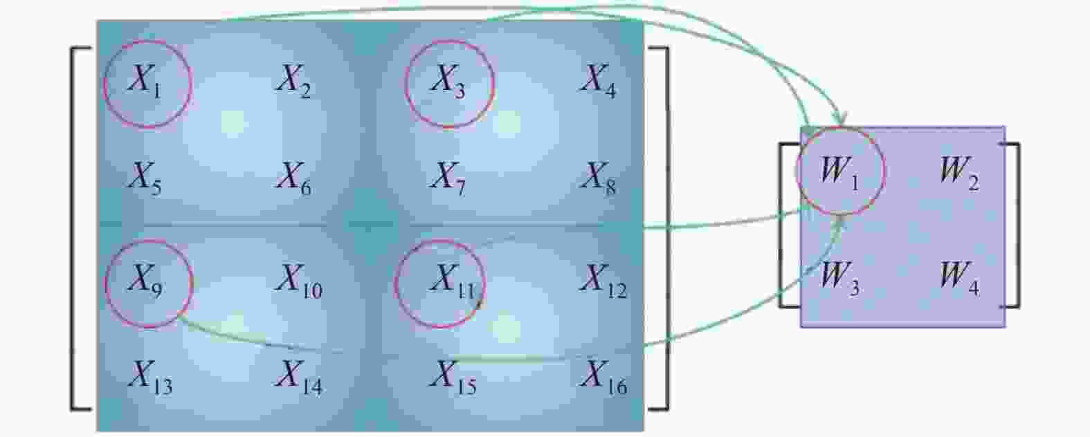
图 2 窗口划分示意图
Figure 2. Diagram of window division
图2中,一个蓝色块窗口的尺寸对应一个微透镜的尺寸。如图1中的红色光线所示,每个窗口内对应位置相同的点,过MLA后出射的光线平行,再经L1后便会汇聚于其焦平面P2上相同的点。P2处接收到的输入图像信息分布可见图3(a),可以在P2处放置强度调制元件(超表面)作为卷积核,其分布如图3(b)所示。

图 3 (a) P2接收到的输入分布; (b) P2处放置的卷积核的形状与数值
Figure 3. (a) The distribution of input signal feed to P2; (b) The shape and value of kernel which set in P2
由于放置的超表面利用不同的透过率分布进行振幅调制,并不会影响光的传播方向。因而之前的匀光操作仅仅是使得共享参数的图像信息叠在一起进行乘法操作。为了再将同窗口经乘法运算后的结果求和,需要让P2处经过处理的光继续沿着原方向传播(P2处仅调制强度,无偏转),再经过光学成像系统做偏转处理。
在L1与L2组成的成像系统中,在P1所在的物方平面处所对应的像方平面放置输出面。假设此处为理想成像系统,物像满足点对点条件。由于物方平面P1处的点为每个窗口内的光线相交而得,因此在像方平面可以实现窗口内求和操作。由于此处设置的成像系统成倒立的实像,所以输出面所得为实际输出分布逆时针旋转180°后的结果。
此处为了使输出面有实像输出,应该使P1所在的物面较后续光学系统(等效于凹透镜)的物距L满足:
$$ L < \frac{{{f_2} \times {f_3}}}{\Delta } $$ (3) -
对于二维输入${\left[ {{{m}},{{n}}} \right]^{\rm{{T}}}}$,经过一个传输矩阵为$ T = \left[ {\begin{array}{*{20}{c}} a&b \\ c&d \end{array}} \right] $的线性无损系统后,输出${\left[ {{{h}},{{k}}} \right]^{\rm{T}}}$。
$$ \left[ {\begin{array}{*{20}{c}} {{h}} \\ {{k}} \end{array}} \right] = \left[ {\begin{array}{*{20}{c}} {{a}}&{{b}} \\ {{c}}&{{d}} \end{array}} \right] \times \left[ {\begin{array}{*{20}{c}} {{m}} \\ {{n}} \end{array}} \right] $$ (4) 因为无损,所以需要满足:
$$ \begin{split} {m^2} + {n^2} = & {h^2} + {k^2} = ({a^2} + {b^2}){m^2} + ({c^2} + {d^2}){n^2} +\\ & 2\left( {ac + bd} \right)mn \end{split} $$ (5) 对于任意的m、n,公式(5)都要成立,因此$\left\{ {\begin{array}{*{20}{c}} {{a^2} + {b^2} = {c^2} + {d^2} = 1} \\ {ac + bd = 0} \end{array}} \right.$,传输矩阵T为酉矩阵。同理,对于其他维度的输入也可以得到此结果。因此,任意线性无损系统的传输矩阵为酉矩阵。
P2处的强度调制操作相当于一衰减片,其传输矩阵为对角矩阵。根据奇异值分解原理,任何矩阵M都可以分解为两个酉矩阵与对角矩阵的乘法($ M = U\Sigma {V^ + } $)。因此,L1,L2与P2组成的系统可以实现任意正值的传输矩阵。
在图1中,使用微透镜阵列将输入图像划分成许多小块,进行并行处理。每一个小块都经历相同的传输矩阵M。将输入的每一个小块做列堆叠,传输矩阵拉成一行,此时图2所示的情况中的输出表示为:
$$ y = \left[ {\begin{array}{*{20}{c}} a&b&c&d \end{array}} \right] \times \left[ {\begin{array}{*{20}{c}} {{X_1}}&{{X_3}}&{{X_9}}&{{X_{11}}} \\ {{X_2}}&{{X_4}}&{{X_{10}}}&{{X_{12}}} \\ {{X_5}}&{{X_7}}&{{X_{13}}}&{{X_{15}}} \\ {{X_6}}&{{X_8}}&{{X_{14}}}&{{X_{16}}} \end{array}} \right] $$ (6) 根据第1节中的公式(2)可知此处实现了卷积运算。
-
对于简单的几何光学系统的仿真,可以利用光线传输矩阵来实现多条光束的追迹。如图4所示,将距离光轴r、角度$\theta $,光强为e的光线表示为${[r,\theta ,e]^{\rm{T}}}$。

图 4 光线标记
Figure 4. Ray marking
根据几何光学的基本定律,易得知光线在均匀介质中的传输矩阵如公式(7)所示,经过薄透镜的传输矩阵如公式(8)所示,以及有一定透过率的强度调制元件的传输矩阵如公式(9)所示。
$$ \left[ {\begin{array}{*{20}{c}} 1&L&0 \\ 0&1&0 \\ 0&0&1 \end{array}} \right] $$ (7) $$ \left[ {\begin{array}{*{20}{c}} 1&0&0 \\ { - 1/{{f}}}&1&0 \\ 0&0&1 \end{array}} \right] $$ (8) $$ \left[ {\begin{array}{*{20}{c}} 1&0&0 \\ 0&1&0 \\ 0&0&{{\tau _{{r}}}} \end{array}} \right] $$ (9) 式中:L为采样距离;${\tau _r}$为距离光轴r处的透射率。对于n条平行入射的光线,将其表示为:
$$ \left[ {\begin{array}{*{20}{c}} r&{r + d}&{...}&{r + (n - 1)d} \\ 0&0&{...}&0 \\ {{e_1}}&{{e_2}}&{...}&{{e_n}} \end{array}} \right] $$ (10) 按照文中所设计的光路,每隔一个采样距离,依次对输入做相应的矩阵操作。需要注意的是,当到达微透镜阵列前表面时,由于此时每个窗口对应的微透镜单元的光轴并非同一个。此处需要加上光轴偏移量如公式(11)所示,再进行矩阵操作(见公式(8))。从微透镜后表面出射时,再减去公式(11),将参照光轴变回同一个主光轴。
$$ \left[ {\overbrace {\begin{array}{*{20}{c}} {\dfrac{n}{{2m}}}&{...}&{\dfrac{n}{{2m}}} \\ 0&{...}&0 \\ 0&{...}&0 \end{array}}^{{m}}\overbrace {\begin{array}{*{20}{c}} {\dfrac{n}{{2m}} - 1}&{...}&{\dfrac{n}{{2m}} - 1} \\ 0&{...}&0 \\ 0&{...}&0 \end{array}}^{{m}}......\overbrace {\begin{array}{*{20}{c}} {\dfrac{{ - n}}{{2m}}}&{...}&{\dfrac{{ - n}}{{2m}}} \\ 0&{...}&0 \\ 0&{...}&0 \end{array}}^{{m}}} \right] $$ (11) 实际仿真时,在强度调制面P2并非直接乘上矩阵(见公式(9)),而是选取r相同的光线的索引,给予相同的透射率,从而制造出强度调制面的矩阵(公式(12)),与入射光线做哈达玛乘积。
$$ \left[ {\begin{array}{*{20}{c}} 1&1&{}&1&1&{}&1 \\ 1&1&{...}&1&1&{...}&1 \\ {{\tau _{r1}}}&{{\tau _{r2}}}&{}&{{\tau _{r1}}}&{{\tau _{r2}}}&{}&{{\tau _{ri}}} \end{array}} \right] $$ (12) 最终,在输出面,由于截断了光线的独立传播,观察到的光强则是相同位置光线强度的叠加。将r相同的光线的e求和,再按照r重新排列。得到输出面的强度分布。
沿着光轴每隔0.5 mm取一个采样面,将所有采样结果记录在数组中,最终按照采样结果仿真出的光路图如图5所示。其中,光强表现在颜色上。仿真结果展示一个卷积核为$\left[ {\begin{array}{*{20}{c}} 0&1&0 \end{array}} \right]$的一维卷积。相同的光路,更改透射率亦可以实现其他卷积核。二维卷积同理。

图 5 仿真光路
Figure 5. Simulate the optical path
-
由于卷积核的大小使用透过率来表示,其值需要约束在0~1,在使用文中的光路做图像锐化时,因为无法实现负的卷积核,需要改变算子的形式。图6为高斯算子(平滑)和Prewitt算子(锐化)应用到超表面后的透射分布以及效果展示。

图 6 (a) 高斯算子;(b) Prewitt算子的变体;(c) Prewitt沿x方向的梯度;(d) 改进的算子沿x方向得到的图像梯度
Figure 6. (a) Gaussian operator; (b) Variant of Prewitt operator; (c) Prewitt's gradient along the x direction; (d) The image gradient obtained by the improved operator along the x direction
当使用此卷积系统实现神经网络的卷积层时,首先在计算机上学习网络所需要的参数。接着根据学习到的卷积核参数,确定超表面需要的透射率分布,再搭建卷积层。
为该系统设计的卷积网络架构如图7所示,空间光调制器SLM1用于加载每层的输入图像,SLM2则用于代替超表面加载卷积核。位于输出面的CMOS相机用于接收每层的输出,再经过计算机处理后将其投到SLM1上用作下一层的输入。同时,将下一层的卷积核更新到SLM2上。反复使用两个SLM用来实现多层卷积。
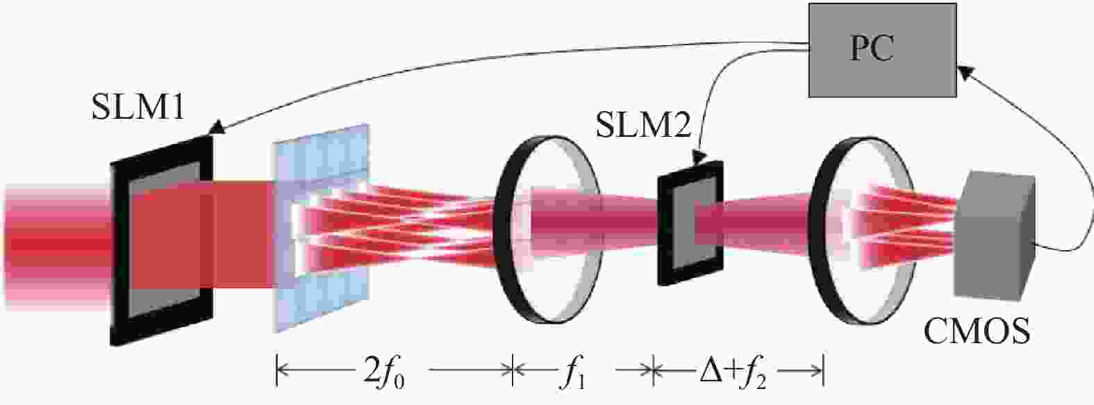
图 7 光学卷积神经网络的示意图
Figure 7. Diagram of optical convolution neural network
在前几节中,描述的卷积系统由于没有对输入做预处理,所实现的卷积的步长只能等于卷积核的尺寸。因而在卷积的同时,也实现了池化,但这样固定的大步长往往会使图像丧失重要的信息。而在图7中描述的光学卷积神经网络,则可以通过计算机对输入到SLM1上的图像做预处理,将卷积核在图片滑动时经过的每个窗口预先划分好,再重排图像投影至SLM1上,从而可以实现各种需要的步长大小和卷积形式。比如图2中所描述的16像素图片,若想实现步长为1的valid卷积,可以将其预处理成图8再投影。同样,若是想实现full或same卷积,可以在一些窗口做补0操作(SLM1上对应的像素点透射率为0)。

图 8 步长为1的valid卷积的预处理结果
Figure 8. Pre-processing result of valid convolution with stride 1
-
文中设计了一款光学系统,基于微透镜阵列与透镜组构成的匀光系统,对光场所携带的图像信息做卷积运算。一方面,可以实现固定的算子做图像模糊或者锐化,用于图像处理系统的预处理;另一方面也可以用作光学卷积神经网络的卷积单元。相较于参考文献[11]中实现一次卷积需要给卷积单元多次加载信息,文中的光学卷积系统仅需加载一次调制信息。然而,由于系统使用透射率作为卷积核的值,只能实现数值范围在0~1的卷积核,这给网络算力带来了上限。在使用SLM投影的有源系统中,可以通过对输入图像的预处理实现各种步长的3种卷积。同一个输入,多次投影卷积核,可以实现多通道输出。同一个卷积核,多通道输入可以同时平铺在输入面。因此,该系统有希望实现多通道的光学卷积神经网络用于一些复杂的图像处理任务。
Optically realize convolution operation of microlens array
-
摘要: 卷积作为一种简单的线性平移不变运算,被广泛应用于图像处理的各个领域,其衍生出的卷积神经网络更是在人工智能领域中大放异彩。为了应对后摩尔时代AI推理芯片算力受限的问题,光学神经网络应运而生。光学卷积神经网络作为其中一个重要的研究热点对光学神经网络的发展起到了重要的推动作用。设计了一种光学卷积系统,基于微透镜阵列与透镜组成的匀光光路对光场所携带的图像做二维卷积,该系统可以光学实现图像平滑和锐化。当使用空间光调制器来投影卷积核和输入图像时,系统可以实现各种步长的三种卷积形式,也可以通过多次投影/平铺实现多通道的三维卷积,进而为实现光学卷积神经网络用于复杂的图像处理任务奠定基础。Abstract: As a simple linear translation invariant operation, convolution has been widely used in various fields of image processing, and the convolutional neural network derived from it is brilliant in the field of artificial intelligence. In order to deal with the problem of limited computing power of AI reasoning chip in the post-Moore era, optical neural network came into being. As one of the important research hotspots, optical convolutional neural network plays an important role in promoting the development of optical neural network. An optical convolution system was designed, based on the uniform light path formed by micro lens array and lens, the image carried in the light place was convoluted in two-dimensions. The system can complete simple image smoothing and sharpening in the optical path. When the spatial light modulator is used to realize the convolution kernel and input surface, the system can realize three convolution forms of various step sizes, and can also realize multi-channel three-dimensional convolution through multiple projection or flattening, thus laying a foundation for the realization of optical convolution neural network for complex image processing tasks.
-
Key words:
- optical convolution /
- microlens array /
- unifying system /
- image processing
-
图 3 (a) P2接收到的输入分布; (b) P2处放置的卷积核的形状与数值
Figure 3. (a) The distribution of input signal feed to P2; (b) The shape and value of kernel which set in P2
图 6 (a) 高斯算子;(b) Prewitt算子的变体;(c) Prewitt沿x方向的梯度;(d) 改进的算子沿x方向得到的图像梯度
Figure 6. (a) Gaussian operator; (b) Variant of Prewitt operator; (c) Prewitt's gradient along the x direction; (d) The image gradient obtained by the improved operator along the x direction
-
[1] Castleman K R, 朱志刚, 林学闵, 等. 数字图像处理[M]. 北京: 电子工业出版社, 1998: 123-145. Castleman K R, Zhu Z, Lin X, et al. Digital Image Processing[M]. Beijing: Publishing House of Electronics Industry, 1998: 123-145. (in Chinese) [2] Goodfellow I J, Bulatov Y, Ibarz J, et al. Multi-digit number recognition from street view imagery using deep convolutional neural networks [J]. arXiv preprint arXiv, 2013, 1312: 6082. [3] 薛珊, 张振, 吕琼莹, 等. 基于卷积神经网络的反无人机系统图像识别方法[J]. 红外与激光工程, 2020, 49(7): 20200154. doi: 10.3788/IRLA20200154 Xue S, Zhang Z, Lv Q Y, et al. Image recognition method of anti UAV system based on convolutional neural network [J]. Infrared and Laser Engineering, 2020, 49(7): 20200154. (in Chinese) doi: 10.3788/IRLA20200154 [4] Long J, Shelhamer E, Darrell T. Fully convolutional networks for semantic segmentation [J]. IEEE Transactions on Pattern Analysis and Machine Intelligence, 2015, 39(4): 640-651. [5] 王中宇, 倪显扬, 尚振东. 利用卷积神经网络的自动驾驶场景语义分割[J]. 光学精密工程, 2019, 27(11): 2429-2438. doi: 10.3788/OPE.20192711.2429 Wang Z Z, Ni X Y, Sheng Z D. Autonomous driving semantic segmentation with convolution neural networks [J]. Optics and Precision Engineering, 2019, 27(11): 2429-2438. (in Chinese) doi: 10.3788/OPE.20192711.2429 [6] Chao D, Chen C L, He K, et al. Learning a deep convolutional network for image super-resolution[C]//ECCV, Springer International Publishing, 2014, 8692: 184-199. [7] 郝建坤, 黄玮, 刘军, 等. 空间变化PSF非盲去卷积图像复原法综述[J]. 中国光学, 2016, 9(1): 41-50. doi: 10.3788/co.20160901.0041 Hao J K, Huang W, Liu J, et al. Review of non-blind deconvolution image restoration based on spatially-varying PSF [J]. Chinese Optics, 2016, 9(1): 41-50. (in Chinese) doi: 10.3788/co.20160901.0041 [8] 朱明, 杨航, 贺柏根, 等. 联合梯度预测与导引滤波的图像运动模糊复原[J]. 中国光学, 2013, 6(6): 850-855. Zhu M, Yang H, He B G, et al. Image motion blurring restoration of joint gradient prediction and guided filter [J]. Chinese Optics, 2013, 6(6): 850-855. (in Chinese) [9] 张旭, 于明鑫, 祝连庆, 等. 基于全光衍射深度神经网络的矿物拉曼光谱识别方法[J]. 红外与激光工程, 2020, 49(10): 20200221. Zhang X, Yu M X, Zhu L Q, et al. Raman mineral recognition method based on all-optical diffraction deep neural network [J]. Infrared and Laser Engineering, 2020, 49(10): 20200221. (in Chinese) [10] 郭玉彬, 邢培. 一种全光模糊智能信息处理系统设计[J]. 光学精密工程, 1998, 6(1): 23-30. doi: 10.3321/j.issn:1004-924X.1998.01.005 Guo Y B, Xing P. The design of an all optical signal processing system with fuzzy intelligence networks [J]. Optics and Precision Engineering, 1998, 6(1): 23-30. (in Chinese) doi: 10.3321/j.issn:1004-924X.1998.01.005 [11] Xu S, Wang J, Wang R, et al. High-accuracy optical convolution unit architecture for convolutional neural networks by cascaded acousto-optical modulator arrays [J]. Optics Express, 2019, 27(14): 19778-19787. doi: 10.1364/OE.27.019778 [12] Mario Miscuglio, Zibo Hu, Shurui Li, et al. Massively parallel amplitude-only Fourier neural network [J]. Optica, 2020, 7(12): 1812-1819. doi: 10.1364/OPTICA.408659 [13] Wu Q, Fei Y, Liu J, et al. High speed and reconfigurable optronic neural network with digital nonlinear activation [J]. Optik, 2021, 247: 168043. doi: 10.1016/j.ijleo.2021.168043 [14] Gu Z, Gao Y, Liu X. Optronic convolutional neural networks of multi-layers with different functions executed in optics for image classification [J]. Optics Express, 2021, 29(4): 5877-5889. doi: 10.1364/OE.415542 [15] Sadeghzadeh H, Koohi S, Paranj A F. Free-space optical neural network based on optical nonlinearity and pooling operations [J]. IEEE Access, 2021, 9: 146533-146549. doi: 10.1109/ACCESS.2021.3123230 -

 点击查看大图

图(8)
计量
- 文章访问数: 495
- HTML全文浏览量: 175
- PDF下载量: 146
- 被引次数: 0

