


 下载:
下载:


-
激光雷达属于主动探测,可通过对激光回波的处理获得相应的目标信息。激光回波的能量与接收口径和脉冲能量息息相关。为了最大限度利用有限的激光回波能量,减少对大口径望远镜、高脉冲能量激光器等硬件的依赖,单光子探测技术得到了越来越多的重视。单光子探测器灵敏度极高,能够探测到非常微弱的光信号[1],显著提升了探测性能,在距离测量等领域展现出了极大的应用潜力。结合时间相关单光子计数技术(TCSPC)[2-8],可在激光回波能量极弱的条件下,根据回波光子在时间上的分布推算得到目标距离,国内外学者对此展开了大量的科学研究。中国科学院大学何巧莹等人基于MPPC阵列开发了一套成像系统,并针对37 m远的目标开展了三维成像实验,在平均每像素累计约1.98个光子的条件下成功对目标进行探测,目标区域测距精度达到0.268 m[9]。南京理工大学的刘驰昊等人分析了影响单光子测距系统测量精度的因素,主要包括激光脉冲强度及回波信号统计脉宽。搭建了实验系统,在10 m远的距离下实现了4 mm的测距精度[10]。赫瑞瓦特大学的Buller等人搭建了一套单光子探测激光雷达系统,采用逐点扫描的方式成功对800 m外的钟塔、6.8 km外的电缆塔、10.5 km外的地形地貌进行了深度测量[11]。中国科技大学的徐飞虎等人利用单光子探测技术,在仅有4个信号光子的条件下,成功对山峰进行测距,绝对距离为162.476 km[12]。
采用逐点扫描方式进行探测的单光子测距激光雷达每次仅能测量一个位置点的信息,无法快速获得大量点云数据。为了提高信号采集效率,麻省理工的Shin等人在发射端将激光发散后对目标进行照明,接收端采用单光子阵列探测器,各像素并行采集回波光子,成功在实验室内对距离4 m左右的人头模型进行了深度测量[13]。近年来,为了提高激光能量的利用率,激光分束照明的方法得到了越来越多的重视。华东师范大学的吴光研究员利用衍射光学元件将一束激光分束成100束,再通过光纤阵列将信号光子接收至1 pixel$ \times $100 pixel的单光子阵列探测器上,以推扫方式成功对500~2500 m的建筑物进行深度测量[14]。月球轨道飞行器激光测高仪利用衍射光学元件将单束激光分成5束,并利用单光子阵列探测器对5束激光的回波光子进行探测,成功对月球表面的地形进行测绘[15]。美国NASA的机载SIMPL激光雷达包含4束激光,激光分为532 nm和1064 nm两种波长,接收端采用阵列探测器并行接收信号光子,并以推扫的方式成功对地形进行测量[16]。2001年,位于马里兰州格林贝尔特的美国国家航空航天局戈达德太空飞行中心开发了一种机载光子计数测距激光雷达。其第二代激光雷达设计用于1 km的飞行高度,发射端利用衍射光学元件以约80%的效率将激光分束成10×10的光束阵列。激光束阵列的回波返回至10$ \times $10分段阳极微通道板光电倍增管的光电阴极上进行数据采集,并在一次飞行实验中成功生成连续的3D图像,空间分辨率达到15 cm[17]。John Degnan曾对多种机载的单光子3D成像激光雷达系统进行了概述总结。其中,由Sigma公司独家资助的HRQLS-2系统将激光分束成10$ \times $10的光束阵列,该激光雷达系统部署在飞机上,具备在3.1 km以上的高度实现高密度探测的能力[18]。
激光分束越多,对激光单脉冲能量的要求越高。为了尽可能地降低激光能量损耗,在不增加激光分束的前提下进一步提高探测的空间分辨率,文中提出了一种旋转扫描与推扫相结合,快速对目标进行探测的方法,可在相同时间内对更多目标点进行测量。旋转扫描导致采样点更加密集并提高了探测的空间分辨率;推扫则使得系统在扫描的方向上能够对更多的目标点进行测量,增加了探测面积。文中所提方法在激光分束的基础上结合了旋转扫描,该方法相较逐点扫描的探测方法,探测的时效性更强;相较激光分束但未结合旋转扫描的方法而言,探测的空间分辨率更高,且在通过旋转扫描所得到的探测点和通过固态分束照明得到的探测点的数量及分布相同的条件下,降低了激光能量损耗。文中所提方法的主要应用场景为激光雷达测绘,在地形测绘、单光子三维成像等领域均有不错的发展潜力。利用单光子阵列探测器搭建实验装置,结合时间相关单光子计数技术对所提方法进行了原理性验证,成功对目标的距离进行测量,并对所搭建系统的测距精准、准确度以及二者与光子计数间的关系进行了探究。
-
文中所提方法结合了推扫和旋转扫描两种扫描方式,以提高光子计数测距激光雷达的探测空间分辨率,如图1所示。发射端将激光分束形成多个照明点以同时对多个目标点进行探测。在推扫的过程中快速旋转分束后的激光,此举可以在短时间内对大量目标点进行扫描,由于旋转后的扫描点分布密集,探测的空间分辨能力将得到提高;接收端采用单光子阵列探测器,并行采集激光回波光子。该方法可在短时间内对大量目标点的数据进行采集,有效提高了探测时效性。该方法相较能够产生同样多采样点或空间分辨能力相同的纯固态激光分束照明的方法而言,所需的激光脉冲能量大幅降低。
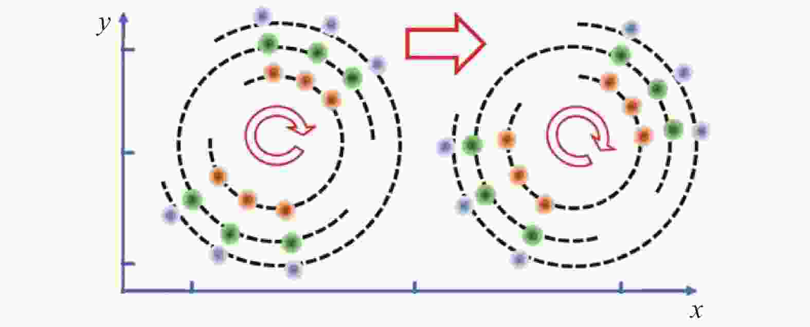
图 1 扫描原理图
Figure 1. Schematic diagram of scanning
假设目标距离为$Z$,光速为$c$,则激光回波光子被探测到的时间在${\text{2}}Z{{/c}}$左右。采用TCSPC技术需保证光子计数小于激光脉冲数的5%[19]。假设测距所需激光回波光子为$\ell $,对应的激光脉冲数应大于$20\ell $,激光脉冲发射总时间应高于$20\ell /f$,其中$f$为激光发射频率。综上可知:旋转扫描的时间间隔应高于$2 Z{\text{/}}c + 20\ell /f$。
-
探测器接收到的光子计数为:
$$ {\lambda _{i,j}}(t) = {\eta _{i,j}}{\gamma _{i,j}}l(t - 2{z_{i,j}}/c) + {\eta _{i,j}}{b_{i,j}} + {d_{i,j}} $$ (1) 式中:$(i,j)$为深度图的像素坐标;${b_{i,j}}$为背景光子通量;${d_{i,j}}$为探测器暗计数率;${z_{i,j}}$为目标距离;$l(t)$为激光脉冲光子通量;$ {\eta _{i,j}} $为探测器的量子效率;${\gamma _{i,j}}$为目标反射率。
假设${T_r}$代表脉冲周期,则一个脉冲周期内的噪声光子数为:
$$ {B_{i,j}} = \int_0^{{T_r}} {({\eta _{i,j}}{b_{i,j}} + {d_{i,j}}} ){\rm{d}}t $$ (2) 一个脉冲周期产生的总信号光子数为:
$$ L = \int_0^{T_r} {l(t)} {\rm{d}}t $$ (3) 假设光子计数为${n_{i,j}}$,一个脉冲周期内探测器接收到的光子数服从泊松分布[20]:
$$ \begin{split} P({n_{i,j}} = k) =& \frac{{\left[{\eta _{i,j}}{\gamma _{i,j}}L + \displaystyle\int_0^{{T_r}} {({\eta _{i,j}}{b_{i,j}} + {d_{i,j}}} ){{{\rm{d}}t}}\right]{^k}}}{{k!}}\cdot\\ & \exp \left[ - ({\eta _{i,j}}{\gamma _{i,j}}L + \int_0^{{T_r}} {({\eta _{i,j}}{b_{i,j}} + {d_{i,j}}} ){{{\rm{d}}t)}}\right] \end{split}$$ (4) 式中:$k$为一个脉冲周期内探测到的光子数。
一个脉冲周期内没有探测到光子的概率为:
$$ {P_0} = P({n_{i,j}} = 0) = \exp [ - ({\eta _{i,j}}{\gamma _{i,j}}L + {B_{i,j}})] $$ (5) 由于探测器具有死区时间,所以单光子探测器在$(0,{T_r}]$内最多仅有一个光子被探测到。故由$N$个激光脉冲所探测到的光子计数${m_{i,j}}$服从二项分布:
$$ P({n_{i,j}} = {m_{i,j}}) = C_N^{{m_{i,j}}}{P_0}^{N - {m_{i,j}}}{[1 - {P_0}]^{{m_{i,j}}}} $$ (6) 由于在笔者的成像系统中,探测器每个脉冲重复周期最多能探测到一个光子,故探测得到的光子到达时间即系统所探测到的第一个光子的到达时间。$W$表示第一个光子的光子到达时间,对于$\forall w \in (0,{T_r})$,给定$(0,{T_r})$中至少有一个光子被探测,$W$的条件分布函数表示为[21]:
$$ \begin{split} F(w) =& P[W \leqslant w|Q(0,{T_r}) \geqslant 1] =\\ & P[Q(0,w) \geqslant 1|Q(0,{T_r}) \geqslant 1] =\\ & \frac{{P[\{ Q(0,w) \geqslant 1\} \cap \{ Q(0,{T_r}) \geqslant 1\} ]}}{{P[Q(0,{T_r}) \geqslant 1]}} =\\ & \frac{{P[Q(0,w) \geqslant 1]}}{{P[Q(0,{T_r}) \geqslant 1]}} =\\ & \frac{{1 - P[Q(0,w) = 0]}}{{1 - P[Q(0,{T_r}) = 0]}} =\\ & \frac{{1 - \exp \left[ - \displaystyle\int_0^w {{\lambda _{i,j}}(t){\rm{d}}t} \right]}}{{1 - {P_0}}} \end{split} $$ (7) 式中:$Q(0,w) = \displaystyle\int_0^w {{\lambda _{i,j}}(t){\rm{d}}t}$;$Q(0,{T_r}) = \displaystyle\int_0^{{{{T}}_r}} {{\lambda _{i,j}}(t){\rm{d}}t}$
根据公式(7)求微分,得到$w$的条件概率密度函数表示为:
$$ {f_W}(w) = \frac{{{\lambda _{i,j}}(w)\exp \left[ - \displaystyle\int_0^w {{\lambda _{i,j}}(t){\rm{d}}t} \right]}}{{1 - {P_0}}} $$ (8) 在低光子通量(可最大限度发挥单光子探测的优势),即$ {\eta _{i,j}}{\gamma _{i,j}}L + {B_{i,j}} \ll 1 $的条件下,忽略公式(8)中的指数部分引入的误差极小。因此,对于像素$(i,j)$,根据任意照明脉冲所探测到的光子而言,光子到达时间的概率密度函数可建模为:
$$ \begin{split} & {f_{{T_{i,j}}}}({t_{i,j}};{\gamma _{i,j}},{z_{i,j}}) = \frac{{{\lambda _{i,j}}({t_{i,j}})}}{{1 - {P_0}}} = \\ & \frac{{{\eta _{i,j}}{\gamma _{i,j}}l({t_{i,j}} - 2{z_{i,j}}/c) + {B_{i,j}}/{T_r}}}{{1 - {P_0}}}\approx \\ & \frac{{{\eta _{i,j}}{\gamma _{i,j}}l({t_{i,j}} - 2{z_{i,j}}/c) + {B_{i,j}}/{T_r}}}{{{\eta _{i,j}}{\gamma _{i,j}}L + {B_{i,j}}}} = \\ & \frac{{{\eta _{i,j}}{\gamma _{i,j}}L}}{{{\eta _{i,j}}{\gamma _{i,j}}L + {B_{i,j}}}}\left(\frac{{l({t_{i,j}} - 2{z_{i,j}}/c)}}{L}\right) + \\ & \frac{{{B_{i,j}}}}{{{\eta _{i,j}}{\gamma _{i,j}}L + {B_{i,j}}}}\left(\frac{1}{{{T_r}}}\right) \\ \end{split} $$ (9) 式中:近似部分得到,在$0 < x \ll 1$的条件下,$1 - {{\rm{e}}^{ - x}} \approx x$。
-
由公式(9)可得到目标深度的最大似然函数为:
$$ \begin{split} \widehat z_{i,j}^{ML} =& \arg \max \prod\limits_{s = 1}^{{n_{i,j}}} {{f_{{T_{i,j}}}}(t_{i,j}^s;{\gamma _{i,j}},{z_{i,j}})} =\\ & \arg \max \sum\limits_{s = 1}^{{n_{i,j}}} {\log \left[{\eta _{i,j}}{\gamma _{i,j}}l\left(t_{i,j}^s - \frac{{2{z_{i,j}}}}{c}\right) + \frac{{{B_{i,j}}}}{{{T_r}}}\right]} \end{split} $$ (10) 式中:$\{ t_{i,j}^s\} _{s = 1}^{{n_{i,j}}}$为光子到达时间数据集。
公式(10)与目标反射率${\gamma _{i,j}}$有关,但对于被探测的目标而言,反射率${\gamma _{i,j}}$不能直接获得,故传统上利用对数匹配滤波估计${z_{i,j}}$[22]:
$$ {\widehat z_{i,j}} = \arg \max \sum\limits_{s = 1}^{{n_{i,j}}} {\log [l(t_{i,j}^s - 2{z_{i,j}}/c)]} $$ (11) -
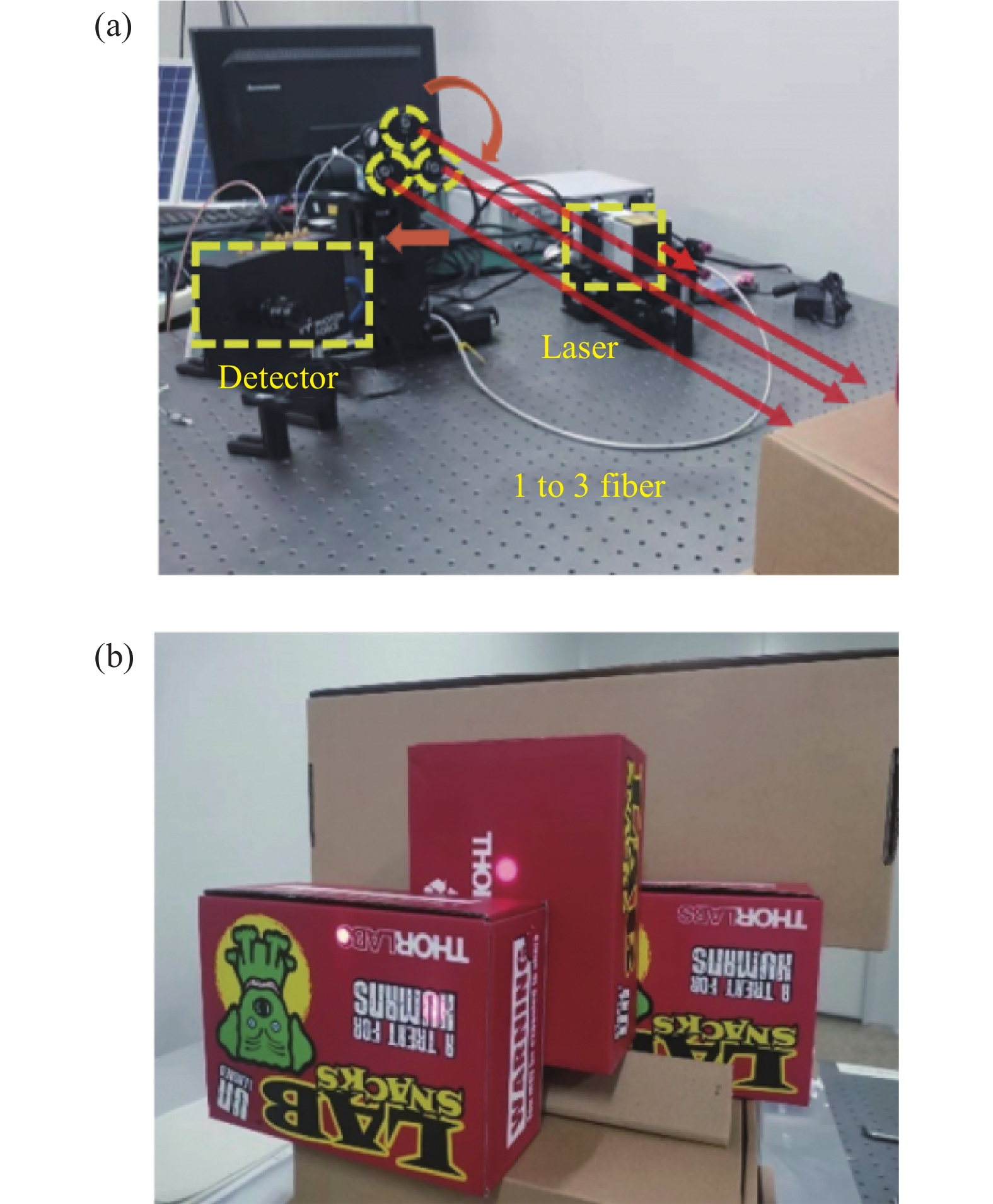
通过信号发生器产生两个同步信号以同步触发激光器及探测器。激光驱动器型号为PicoQuant公司生产的Taiko PDL M1,激光头型号为LDH-IB-640-B,激光波长为637.5 nm,功率可调,最大值为7.1 mW,实验时调制至最大功率的10%。激光器发射脉冲激光,脉冲频率为20 MHz,激光脉宽为480 ps。探测器型号为Photon Force公司生产的PF32,包含1024个像素,每个像素均单独集成有计时器,精度为55 ps,探测器在激光器波段的量子效率为23%。探测器具有光子计数及时间相关单光子计数两种工作模式,实验时选择后者。定制1分3的可见光波段多模光纤LWS-1MIR200FF,将激光耦合进该光纤的单光纤头,利用该光纤将激光分成3束,通过旋转光纤支架来旋转激光束群并以此模拟旋转扫描的过程,将支架固定在电动位移平台GCD-203300M上,通过该平台对支架进行平移以模拟推扫过程。激光照射至目标后,反射回的信号光子由单光子阵列探测器进行接收并处理。实验装置及目标见图2(a),目标见图2(b)。
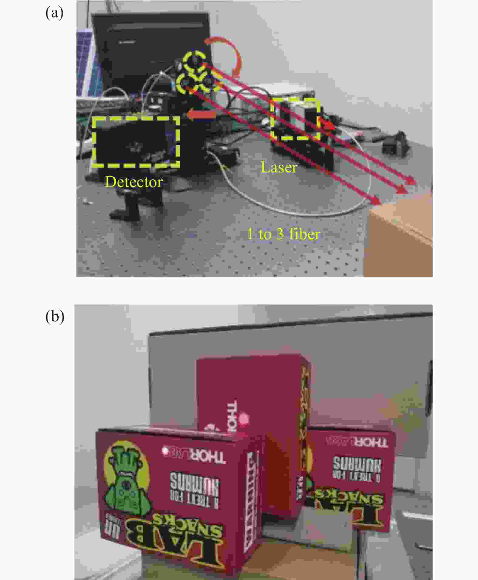
图 2 实验光路图及目标图。(a)光路图;(b)目标图
Figure 2. Experimental optical path image and target image. (a) Optical path image; (b) Target image
-
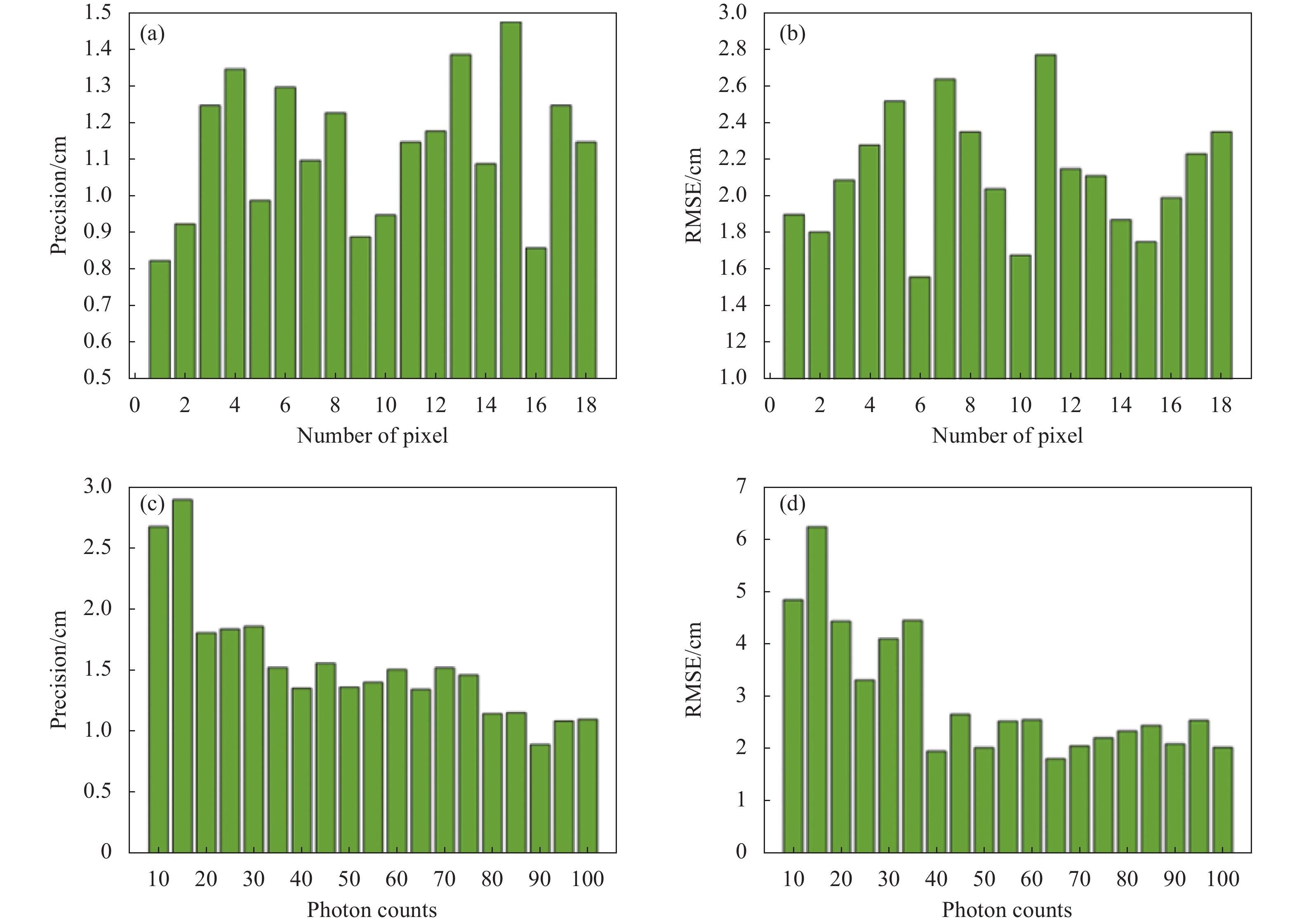
文中探究了目标点对应中心像素处的测距精度(precision)与测距准确度(accuracy)两个性能指标,为所搭建的激光雷达系统能够准确测量目标距离的可行性提供了支撑。利用光纤将激光分成3束,对目标进行照明并利用单光子阵列探测器并行采集信号光子,数据采集完成后将光纤支架旋转30°以模拟旋转扫描,旋转后再次采集数据;旋转后利用电动位移台移动光纤支架以模拟推扫,并采集信号光子数据,如此重复,共采集得到18个目标点数据。在每一个目标点上重复采集50组数据并分别计算得到50组目标距离,以测得各组距离的标准差作为激光雷达系统的测距精度[10];将测量得到的各组距离与真实距离间的均方根误差(RMSE)作为测距准确度[13]。RMSE的计算公式为:
$$ {{RMSE}} = \sqrt {\frac{1}{\mu }\sum\limits_{j = 1}^\mu {{{({R_j} - R)}^2}} } $$ (12) 式中:$\;\mu $为根据数据计算得到的距离数量;${R_j}$代表计算得到的第$j$个距离值;$R$为目标真实距离。
根据实验数据,计算得到的各目标点对应像素处的测距精度如图3(a)所示,测距准确度如图3(b)所示。以阵列探测器的单个像素所采集的激光回波光子数据为例,探究测距精度及准确度与光子计数之间的关系。激光对目标进行照明后,利用单光子探测器采集信号光子数据,改变探测器采集时间进而改变探测光子数,各个探测光子条件下均重复采集30组数据,进而计算得到不同光子计数条件下的测距精度及准确度,分别如图3(c)及图3(d)所示。可见,当光子计数不断增加时,系统测距精度及准确度逐渐提高直到趋于一个常数。

图 3 测距系统性能指标。(a)测距精度;(b)测距准确度;(c)不同光子计数下的测距精度;(d) 不同光子计数下的测距准确度
Figure 3. Performance index of ranging system. (a) Ranging precision; (b) Ranging accuracy; (c) Ranging precision at different photon counts; (d) Ranging accuracy at different photon counts
为进一步研究目标位置对测距精度及准确度的影响,进行了如下实验:以阵列探测器单像素所测距离信息为例,激光发射照明目标,信号光子在目标表面发生漫反射,利用单光子探测器对反射回的光子数据进行采集。每次采集过后将目标向后移动3 cm以改变目标位置,再改变探测器采集时间以改变探测光子数,在各个目标位置及各个光子计数的条件下重复采集30组光子数据,进而计算得到探测光子数分别为20、60、100时,在不同位置的测距精度及准确度,分别如图4(a)及图4(b)所示。由此可见,测距精度及准确度与光子计数间的关系与目标所处位置无关。
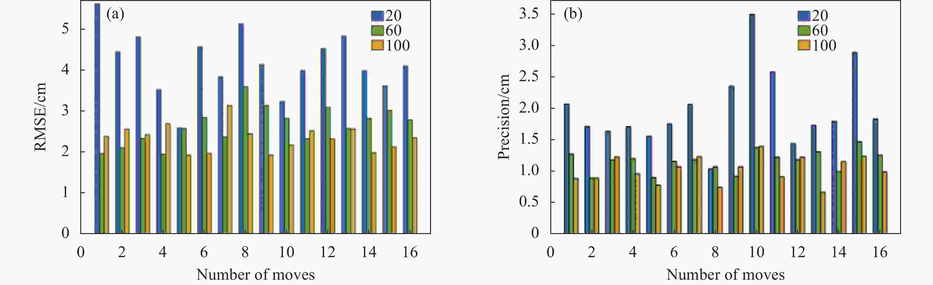
图 4 (a)不同距离、不同光子计数条件下的测距准确度;(b)不同距离、不同光子计数条件下的测距精度
Figure 4. (a) Ranging accuracy under different distances and different photon counts; (b) Ranging precision under different distances and different photon counts
-
利用光纤将激光分成3束,分束后的激光对目标进行照明,利用单光子探测器采集一组数据并对目标距离进行测量后,旋转激光束群,再次采集数据并测距;利用位移平台移动光纤,重复上述过程,共得到18个目标点的距离信息。激光回波在探测器上的分布如图5(a)~(f)所示,其中颜色条代表光子计数值。采用时间相关单光子计数技术,根据光子到达时间统计数据对扫描得到的18个目标点的距离进行测量,结果如图5(g)所示。

图 5 (a)~(f) 激光回波在探测器上的分布;(g)各个目标点所测得的距离
Figure 5. (a)-(f) Distribution of laser echo on array detector; (g) Distance measured at each target point
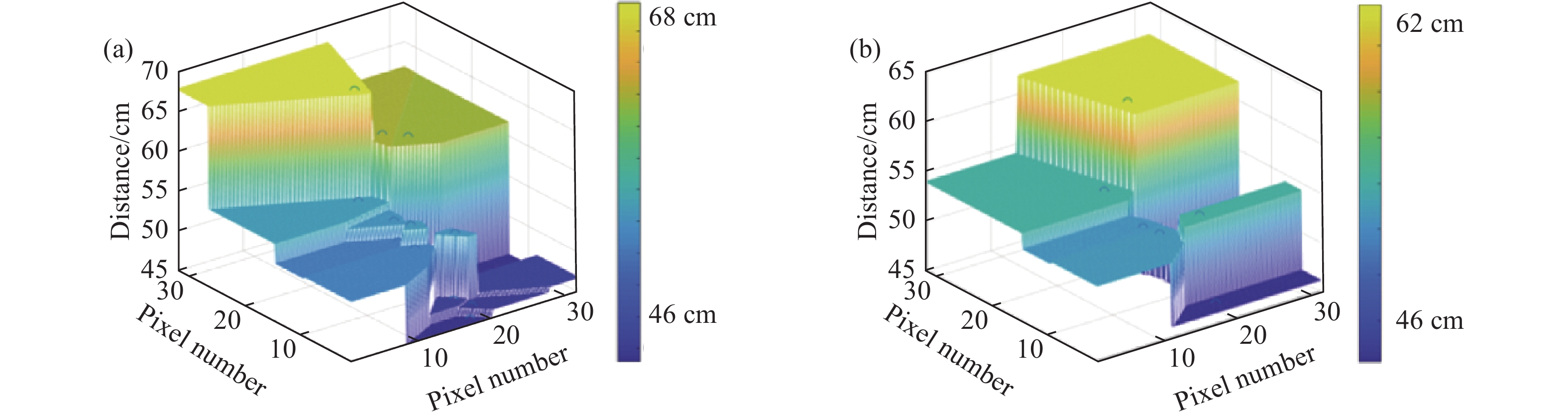
图6为采用激光分束的方法进行探测形成的距离图,颜色条表示目标点距离。相较逐点扫描的方法,激光分束照明法单位时间内可探测的目标点数提高了$b$倍,进而提高探测时效性,其中$b$为分束后激光的数量,图6中$b$值为3。实验中增加了旋转扫描,成功对多个目标点进行测距,根据各个目标点的距离采用插值的方法恢复出目标的三维特征,如图6(a)所示,忽略掉测量误差共显示出4个距离特征。根据不采用旋转扫描所测得的目标点距离恢复出的目标如图6(b)所示,忽略掉测量误差共显示出3个距离特征。可见,由于增加了旋转扫描,使得激光照射到了未经旋转扫描的探测方式所照射不到的目标点位置,多测量出一个距离特征,以文中所得实验数据为例,增加了33%的距离特征量。图6(a)增加了旋转扫描,在旋转速度足够快的条件下,单位时间内探测到的空间分辨率较不经旋转扫描的方法,如图6(b)所示,有所提高。同时,文中所提出的基于旋转扫描的探测方式相较未经过旋转扫描的方式而言,在探测目标点总数量及分布相同的条件下(空间分辨率相同),激光能量损耗降低至$1/(a + 1)$,其中$a$代表旋转次数。

图 6 (a)经过旋转扫描测得的目标深度信息图;(b)未经旋转扫描测得的目标深度信息图
Figure 6. (a) Target depth information map measured by rotary scanning; (b) Target depth information map without rotary scanning
受实验条件所限,文中将激光分束至3束,且可旋转角度较少;在后续的研究中,将增加激光分束数量,并提高可旋转角度的灵活性,以提高探测点的数量及密度,并对发射端各部件进行集成,进而提高激光探测的空间分辨率并优化系统的发射端结构。
-
文中提出了一种新的高效率光子计数测距激光雷达,该系统对目标深度特征的高空间分辨率探测起到了一定的推进作用。将激光分束以探测多个目标点,为扩大探测面积,采用推扫的方式将激光束群照射到目标的其他位置;在推扫的过程中,快速旋转激光束群,在相同时间内便可测得更密集的扫描点的距离。在提高探测时效性的同时,也提高了探测的空间分辨率,使得目标在空间上的深度特征更加明显。同时,较纯固态激光分束照明方法,激光总能量消耗降低。搭建实验系统成功进行了原理验证,测得距离信息较未经算转扫描所得信息增加了33%。对系统的测距精度及准确度进行了测量,系统测距精度优于1.48 cm,准确度优于2.78 cm。且二者数值均随着光子数成负相关关系,直至趋于不变,此规律与目标位置无关。可见文中所提方法,具有高时效性,分束激光总能量低,高探测空间分辨率等优点,在具有空间二维特征的目标的距离探测上具有应用潜力。
High resolution photon counting ranging method based on rotary scanning
-
摘要: 光子计数测距激光雷达在暗弱目标探测、激光遥感等方面均有着极大的应用潜力。激光固态密集分束照明探测虽然相较逐点扫描的方法而言,能够有效提高探测时效性,但在保证较高探测空间分辨率的条件下,激光能量损耗较大。为了能够既保证对目标的高效探测,同时减少密集分束对激光能量的消耗,提出了旋转扫描与推扫相结合的探测方法。对目标进行激光分束照明后,在推扫的过程中快速旋转激光束群,并利用单光子阵列探测器同时对不同目标点返回的信号光子进行采集,以此在固定时间内得到更多的采样点数据。搭建单光子测距系统,发射端利用光纤将激光进行分束,利用位移台模拟推扫,旋转光纤支架模拟旋转扫描,接收端通过单光子阵列探测器并行接收回波光子。对文中所提方法进行了原理性验证,测量出系统测距的精度和准确度,并对上述二者与光子计数间的关系进行了探究。实验结果表明:对于文中所搭建系统,目标点所在像素位置测距的精度优于1.48 cm,准确度优于2.78 cm。二者均随着光子数的增加而提高,并逐渐趋于一个常数。经过旋转扫描,所测得的深度信息较未经旋转扫描所测深度信息增加了33%。总结可得通过旋转扫描能够有效提高探测得到的目标空间分辨率。Abstract:
Objective Owing to the large loss of the laser during the transmission process, the echo signal light is weak when the target is faint; Therefore, the requirements for the single pulse energy of the laser and the aperture of the telescope are extremely high. Photon counting detection has the advantage of high sensitivity, and can detect weak echo signals. By combining the two technologies of single-photon detection and time-correlated single-photon counting (TCSPC), laser energy consumption and telescope aperture size can be significantly reduced when detecting faint targets. Photon counting ranging lidar has great application potential in faint target detection and laser remote sensing, etc. Although detection method using solid-state dense beam splitting laser illumination can effectively improve detection timeliness compared to point-by-point scanning methods and ensure high detection spatial resolution, laser energy loss is significant. In order to ensure the efficient detection of targets and reduce the consumption of laser energy caused by dense beam splitting, a detection method combining rotary scanning and push scanning was proposed. In order to better understand the influencing factors of photon counting ranging, the relationship between the above two and photon counts was explored. Methods A single-photon ranging system was built. After illuminating the target by laser beam splitting method, which divides the laser into three beams using optical fibers, a single-photon array detector is used to collect signal photons from different target points in parallel (Fig.2). After data collection is completed, the optical fiber bracket is rotated 30° to simulate rotational scanning, and signal-photon counting is collected again. After rotation, an electric displacement table is used to move the fiber optic bracket to simulate scanning, and signal-photon counting data is collected. This process is repeated to collect a total of 18 target point data. 50 sets of data are collected repetitively at each target point, using the standard deviation of the measured distances as the ranging accuracy of the LiDAR system; The root mean square error (RMSE) between the measured distances and the true distance is used as the ranging accuracy. Taking the laser echo photon data collected by a single pixel of an array detector as an example, the relationship between ranging accuracy and photon counting is explored. After illuminating the target, a single-photon detector is used to collect signal-photon data, changing the acquisition time of the detector to change the number of detection photons. Under each detection photon condition, 30 sets of data are repeatedly collected, and then the ranging accuracy and precision under different photon counting conditions are calculated. To further investigate the impact of target position on ranging accuracy and accuracy, after each acquisition, the target is moved back 3 cm to change the target position, and then the detector acquisition time is changed to change the number of detected photons. Under the conditions of each target position and photon count, 30 sets of photon data are repeatedly collected, and the ranging accuracy at different positions are calculated under different photon counts. Based on the measured distance values of 18 target points, the three-dimensional features of the target are restored using interpolation method. And the 3D image of the target recovered from rotating scanning detection is compared with the 3D image recovered from without rotating scanning to demonstrate the feasibility of using rotating scanning for high spatial resolution detection. Results and Discussions The ranging precision and accuracy at the pixels corresponding to the target points are calculated for the system built in the experiment. Ranging precision and accuracy decrease with the increase of the number of photons and gradually tend towards a constant (Fig.3). Their relationship with photon counts is independent of the target position (Fig.4). The depth information measured after rotary scanning increased by 33% compared to the depth information measured without rotary scanning (Fig.6). It can be concluded that the method with rotating scanning can effectively improve the spatial resolution of the detected target. Meanwhile, compared to the method without rotating scanning, the detection method based on rotating scanning reduces the laser energy loss under the condition that the total number and distribution of detected target points are the same. Conclusions A new high-efficiency photon counting ranging lidar is proposed, which plays a certain role in promoting the high spatial resolution detection of target depth features. The laser beam is splitted to detect multiple target points, and push scanning is used to expand the detection area; During the push scanning process, the laser beam group is quickly rotated to measure the distance of more dense scanning points within the same time. While improving the timeliness of detection, it also improves the spatial resolution of detection, making the depth characteristics of the target more obvious in space. Meanwhile, compared to pure solid-state laser beam splitting illumination methods, the total laser energy consumption is reduced. And the distance information of the target increased compared to the distances obtained without rotary scanning. The ranging accuracy and accuracy of the system were measured, and the ranging accuracy was better than 1.48 cm and the accuracy was better than 2.78 cm. And both values are negatively correlated with the number of photons until they tend to remain unchanged, which is independent of the target position. The proposed method has advantages such as high timeliness, low total energy, and high detection spatial resolution, and has application potential in distance detection of targets with spatial two-dimensional features. -
Key words:
- photon counting /
- lidar /
- laser ranging /
- rotary scanning
-
图 2 实验光路图及目标图。(a)光路图;(b)目标图
Figure 2. Experimental optical path image and target image. (a) Optical path image; (b) Target image
图 3 测距系统性能指标。(a)测距精度;(b)测距准确度;(c)不同光子计数下的测距精度;(d) 不同光子计数下的测距准确度
Figure 3. Performance index of ranging system. (a) Ranging precision; (b) Ranging accuracy; (c) Ranging precision at different photon counts; (d) Ranging accuracy at different photon counts
图 4 (a)不同距离、不同光子计数条件下的测距准确度;(b)不同距离、不同光子计数条件下的测距精度
Figure 4. (a) Ranging accuracy under different distances and different photon counts; (b) Ranging precision under different distances and different photon counts
图 5 (a)~(f) 激光回波在探测器上的分布;(g)各个目标点所测得的距离
Figure 5. (a)-(f) Distribution of laser echo on array detector; (g) Distance measured at each target point
-
[1] 邬京耀, 苏秀琴, 镡京京, 等. 基于单光子阵列探测器的隐藏目标瞬时成像理论研究 [J]. 红外与激光工程, 2018, 47(S1): 105-111. Wu Jingyao, Su Xiuqin, Tan Jingjing, et al. Study of theory for transient imaging of hidden object using single-photon array detector [J]. Infrared and Laser Engineering, 2018, 47(S1): S122002. (in Chinese) [2] Mccarthy A, Krichel N J, Gemmell N R, et al. Kilometer-range, high resolution depth imaging via 1560 nm wavelength single-photon detection [J]. Optics Express, 2013, 21(7): 8904-8915. doi: 10.1364/OE.21.008904 [3] Bao Z, Liang Y, Wang Z, et al. Laser ranging at few-photon level by photon-number-resolving detection [J]. Applied Optics, 2014, 53(18): 3908-3912. doi: 10.1364/AO.53.003908 [4] Maccarone A, Mccarthy A, Ren X, et al. Underwater depth imaging using time-correlated single-photon counting [J]. Optics Express, 2015, 23(26): 33911-33926. doi: 10.1364/OE.23.033911 [5] Liang Y, Huang J, Ren M, et al. 1550-nm time-of-flight ranging system employing laser with multiple repetition rates for reducing the range ambiguity [J]. Optics Express, 2014, 22(4): 4662-4670. doi: 10.1364/OE.22.004662 [6] Ren M, Gu X, Liang Y, et al. Laser ranging at 1550 nm with 1-GHz sine-wave gated InGaAs/InP APD single-photon detector [J]. Optics Express, 2011, 19(14): 13497-13502. doi: 10.1364/OE.19.013497 [7] Cao R, Xu J, Yang C, et al. High-resolution non-line-of-sight imaging employing active focusing [J]. Nat Photonics, 2022, 16(6): 462-468. doi: 10.1038/s41566-022-01009-8 [8] Li Z, Huang X, Cao Y, et al. Single-photon computational 3D imaging at 45 km [J]. Photonics Research, 2020, 8(9): 1532-1540. doi: 10.1364/PRJ.390091 [9] 何巧莹, 黄林海, 顾乃庭. 基于MPPC阵列的三维单光子成像技术研究 [J]. 红外与激光工程, 2022, 51(10): 20210989. doi: 10.3788/IRLA20210989 He Qiaoying, Huang Linhai, Gu Naiting. 3D single photon imaging technology research based on MPPC array [J]. Infrared and Laser Engineering, 2022, 51(10): 20210989. (in Chinese) doi: 10.3788/IRLA20210989 [10] 刘驰昊, 陈云飞, 何伟基, 等. 单光子测距系统仿真及精度分析 [J]. 红外与激光工程, 2014, 43(2): 382-387. doi: 10.3969/j.issn.1007-2276.2014.02.008 Liu Chihao, Chen Yunfei, Gu Naiting, et al. Simulation and accuracy analysis of single photon ranging system [J]. Infrared and Laser Engineering, 2014, 43(2): 382-387. (in Chinese) doi: 10.3969/j.issn.1007-2276.2014.02.008 [11] Pawlikowska A M, Halimi A, Lamb R A, et al. Single-photon three-dimensional imaging at up to 10 kilometers range [J]. Optics Express, 2017, 25(10): 11919-11931. doi: 10.1364/OE.25.011919 [12] Li Z, Ye J, Huang X, et al. Single-photon imaging over 200 km [J]. Optica, 2021, 8(3): 344-349. doi: 10.1364/OPTICA.408657 [13] Shin D, Xu F, Venkatraman D, et al. Photon-effificient imaging with a single-photon camera [J]. Nat Communication, 2016, 7(1): 12046-12046. doi: 10.1038/ncomms12046 [14] Li Z, Wu E, Pang C, et al. Multi-beam single-photon-counting three-dimensional imaging lidar [J]. Optics Express, 2017, 25(9): 10189-10195. doi: 10.1364/OE.25.010189 [15] Araki H, Tazawa S, Noda H, et al. Lunar global shape and polar topography derived from Kaguya-LALT laser altimetry [J]. Science, 2009, 323(5916): 897-900. doi: 10.1126/science.1164146 [16] Harding D, Dabney P, Abshire J, et al. The slope imaging multi-polarization photon-counting lidar: an advanced technology airborne laser altimeter [R]. NASA Earth Science Technology Forum, 2010: 253–256. [17] John D. Photon counting lidars for airborne and spaceborne topographic mapping [C]//Applications of Lasers for Sensing and Free Space Communications, 2010. [18] John D. Scanning, multiple, single photon lidars for rapid, large scale, high resolution, topographic and bathymetric mapping [J]. Remote Sensing, 2016, 8(11): 958. doi: 10.3390/rs8110958 [19] Rapp J, Ma Y, Goyal V K, et al. High-flux single-photon lidar [J]. Optica, 2021, 8(1): 30-39. doi: 10.1364/OPTICA.403190 [20] Snyder D L. Random point processes [J]. Journal of the Royal Statistical Society, 1975, 139: 990. [21] Huang P, He W, Gu G, et al. Depth imaging denoising of photon-counting lidar [J]. Applied Optics, 2019, 58(16): 4390-4394. doi: 10.1364/AO.58.004390 [22] Shin D, Kirmani A, Goyal V K, et al. Photon-efficient computational 3-D and reflectivity imaging with single-photon detectors [J]. IEEE Trans on Computational Imaging, 2015, 1(2): 112-125. doi: 10.1109/TCI.2015.2453093 -

 点击查看大图

计量
- 文章访问数: 74
- HTML全文浏览量: 46
- PDF下载量: 33
- 被引次数: 0

