自由空间光通信(Free Space Optical Communication, FSO)，又称大气激光通信，是一种以激光束为载体，大气为传输介质，实现高速传输的无线通信方法，具有传播速率高、可用带宽大、无需频率许可、抗电磁干扰能力强、保密安全性好、激光终端体积小、质量轻和功耗低等优点^[1]。但是，当光信号在自由空间传输时，由于温度和气压的不均匀变化，容易受到大气湍流的影响，比如光强闪烁、相位漂移和光束扩等展^[2-3]，严重影响了FSO系统的通信性能。

卫星激光通信是自由空间光通信的最新应用，它是利用人造地球卫星作为中继站转发或发射信号，在卫星通信地球站之间或者地球站与航天器之间进行的通信。星地通信是卫星通信的重要组成部分，包括卫星对地面站的下行链路与地面站对卫星的上行链路，在星地激光通信的过程中，携带信息的光载波会穿过地球表面的大气层。与近地FSO相比，星地激光通信具有覆盖面积大、通信距离远、不受地理条件限制、地面站可以建在偏远地区，如海岛、大山、沙漠、丛林等地形地貌复杂区域等优点，这对真正实现在任何时间、任何地点都能便捷地获得和交流信息都至关重要^[4-5]。

对于星地激光大气的长距离传输，现有的解析理论无法对光传输特性给出清晰的描述，而外场远距离激光大气传播实验存在实验参数不可控、重复性差等缺点，同时实验链路的传输距离有限，其光强测试结果与实际星地链路实验结果仍需评估。因此，为了预测卫星光学接收器孔径处的波前行为，以便充分预测通信链路预算和确定光学系统的设计要求，数值仿真成为评估大气湍流对光束传输影响的一个有效途径。

在现有的星地激光传输的仿真中，都是基于均匀的湍流环境，大气湍流都是采用Kolmogorov谱模型。文献[6]建立了Kolmogorov谱下的激光传输模型，模拟了地面终端与卫星之间的上行通信，利用了18层相位屏来模拟20 km以下的大气湍流，分析了不同湍流度或天顶角下的光强闪烁指数^[6]。钱仙妹等人针对地空激光大气的长距离斜程传输进行了大量数值模拟，通过变化天顶角 、光束初始半径和激光长等传输条件 ，等量分析了光束有效半径以及光束能量的变化^[7]。最近的研究表明，在距离地面大于2 km的区域，大气湍流与传统的Kolmogorov模型有偏差，主要是湍流的谱指数不在于固定的11/3，而是3~5之间变化，与高度有关^[8]。对于地-星和星-地数据链激光通信系统，其湍流路径至少有20 km，大气占信道很大一部分，性能的估计主要依赖于传播预测代码中使用的大气湍流模型的精度，因此使用传统的Kolmogorov谱将会产生误差。另一方面，现有的数值仿真采用的相位屏数量多，计算机运行时间长，并不适用星地链路间复杂的湍流环境。近年来，基于Non-Kolmogorov 湍流光传播得到了广泛研究，研究人员分析了不同类型的光束在Non-Kolmogorov湍流中的各种传播效应。2010年，Shchepakina等人通过数值计算，分析了高斯-谢尔模型(EMGSM)波束在具有不同的谱幂律的Non-Kolmogorov湍流中传输的二阶统计量，发现湍流对传播光束的影响主要取决于Non-Kolmogorov的谱幂律$ \alpha $^[9]。2012年，Italo Toselli等人研究了上行和下行路径激光束通过Non-Kolmogorov湍流传播的性能，推导了高斯光束长期波束半径的解析形式，数值仿真了平面波与球面波的闪烁指数随谱幂律$ \alpha $变化曲线^[10]。2017年，Chen等人采用高斯分布描述沿传播路径的幂律，提出了基于等效折射率结构常数的Non-kolmogorov湍流模型，通过数值仿真，分析了Non-kolmogorov湍流对高斯光束传输的影响^[11]。不过大多数相关研究都假设传播路径上的湍流功率谱的幂律相同，然而实际情况下，这种假设并不成立，因为传播路径上的湍流功率谱幂律具有随机波动性。假设传播路径上的湍流功率谱幂律相同得出的所谓的Non-Kolmogorov湍流传播效应，可能缺乏实际参考价值。基于Non-Kolmogorov谱的星地大气湍流的研究还处于理论分析阶段^[12-13]，相应的数值仿真很少。2010年，Du等人进行了对流层Kolmogorov湍流和平流层Non-Kolmogorov湍流对卫星激光通信的联合影响研究，分析了上行链路和下行链路的长期光束扩展、闪烁指数以及误码率等。2014年，熊准基于LC-SLM设计了室内湍流模拟器并搭建了仿真平台，分析了Kolmogorov与Non-Kolmogorov湍流中不同湍流强度下的光束到达角起伏情况，并在此基础上介绍了一种卫星光通信终端地面演示系统，该系统可用于链路预算分析^[14]。

在数值仿真中，模拟湍流的相位屏数量太多会增加系统的复杂度。为了尽可能接近仿真结果同时降低复杂度，文中以地面站对卫星的上行传输为背景，考虑链路长距离且不均匀的湍流环境，通过计算数值仿真的约束条件，提出了3层传输仿真模型。为了验证模型的准确性，对比了传统的Kolmogorov谱下相位屏为2层、3层、6层、11层以及21层时观测面光场的互相干因子，并将其与理论值比较，证明了3层模型的可行性。同时考虑到地对卫星链路不均匀的湍流环境，基于3层模型，对比了Kolmogorov谱与Non-Kolmogorov谱下光束传输的仿真结果。

近20年来，研究者对大气湍流折射率的性质表现出了极大地兴趣，提出了各种理论模型来研究其特性。其中，针对Kolmogorov谱的分析最为广泛，Kolmogorov的湍流理论认为，对于局域均匀且各向同性的大气湍流，存在一个惯性区域，该区域的折射率波动的特征可以用大气湍流折射率谱密度函数${{{\varPhi }}_n}\left( {{k_r}} \right)$来描述，其中${k_r} = {{2\pi }}/{\lambda }$是空间波函数，单位为$ {{\rm{m}}}^{-1}，\lambda $表示光波长。Kolmogorov谱可以适用于绝大多数近地FSO系统，其具体表达式为^[15]：

式中：11/3为低空湍流谱指数；${L_0}$为折射率波动的外部相关长度，称为外尺度；${l_0}$为内尺度，表示内部相关长度^[16]；$C_n^2$为折射率结构常数，是大气光学中的一个非常重要的参数，它描述了大气折射率起伏的强度，可以用它来表示湍流的强弱。在近地面的FSO系统中，大气湍流在传输路径上是均匀分布的，即同一时刻大气折射率结构常数$C_n^2$在整条传输链路上保持不变^[3]。

而在地星链路上，激光传输贯穿整个大气层，需要采用大气折射率结构常数的海拔分布模型，即$C_n^2\left( h \right)$。Hufnagel-Valley在实测的基础上，根据实验数据，提出了大气湍流强度$C_n^2$随高度变化的模型，表示为^[17]：

式中：$h$为距离地面的海拔高度；$v\left( {{\rm{m}}/{\rm{s}}} \right)$为均方根风速。当$A = 1.7 \times {10^{ - 14}}\left( {{{\rm{m}}^{ - {2}/{3}}}} \right)$，$v = 21\left( {{\text{m}}/{\rm{s}}} \right)$ 时称为Hufnagel-Valley 5/7模型，可以用来表示白天的大气湍流强度随高度的变化，该模型被广泛地应用于大气湍流仿真建模研究中^[18]。因此，文中有关大气湍流强度的计算也是基于该模型。

高层大气中，Kolmogorov谱不能正确地描述大气湍流统计^{[12, 19-20]}，特别是在垂直传输路径上，湍流是不均匀的，其湍流谱的谱指数也随高度变化^[19]，而不是固定的11/3。也就是说，无论是在近地面受地面因素影响明显的情况下还是在高空自由的大气中，大气湍流大都与各向同性特性有一定的偏离，任何偏离局地均匀各向同性的湍流都可称为Non-Kolmogorov湍流。大气湍流的功率谱指数在不同的高度、气压、温度和湿度等因素下可能会有所不同，通常来说，随着高度的增加，大气湍流的功率谱指数会逐渐减小^[21]。

Zilberman等人将卫星激光通信的大气信道看作是由地面到2 km的Kolmogorov湍流、2~10 km的谱指数为10/3的Non-Kolmogorov湍流以及10 km以上谱指数为5的Non-Kolmogorov湍流组成，同时给出了在该模型下谱指数随高度变化的表达式^[22]:

式中：$ {\alpha _1} $、$ {\alpha _2} $和$ {\alpha _3} $分别为边界层、对流层和平流层内的湍流谱指数；${{{H}}_1}$和${{{H}}_2}$为大气层边界；$ {b_1} $和$ {b_2} $为层间平滑系数。

但是，该模型的准确性尚未得到验证，实际上，具体的谱指数随高度的变化趋势可能因不同的环境条件和研究区域而有所不同，因此文献[22]中的湍流谱模型不具有普适性，具体的研究需要依据实际情况和观测数据来确定。根据现有的测量与实验研究，自由对流层中的湍流比平流层中更加强烈，以我国青藏地区和青海湖地区为例，青藏地区边界层的谱指数在2.4~2.7之间，自由对流层的谱指数大约在2.9~3.1之间，平流层的谱指数大约在2.9~2.7之间^[23]。青海湖地区在低空、中空和高空的谱指数则分别为3.67、3.47和3.20^[24]。

因此，文中采用可以表示任意谱指数的Non-Kolmogorov湍流折射率波动的三维功率谱模型 ，不考虑湍流内外尺度时，具体地表达式如下^{[12, 25-26]}：

式中：$\; \beta \left(h\right) $为Non-Kolmogorov谱的折射率结构常数，是随高度和湍流谱指数变化的参数，与$C_n^2\left( h \right)$的关系为：

式中：$L$为总传输距离。

分步传输算法（split-tep beam propagation method）被广泛的用于光束在随机介质中的数值仿真。主要原理是将光在随机介质中的传输分解成一段段真空与相位屏的共同作用。当传输距离$ \Delta z $大于外尺度$ {L_0} $时，可以将公式（4）空间折射率谱${\varPhi _n}\left( {{k_r},h,\alpha } \right)$写成路径依赖的形式：

式中：$ \displaystyle\int_{{z_i}}^{{z_{i + 1}}} {\sigma _n^2\left( z \right){\rm{d}}z} $为传输距离$ \left[ {{z_i},{z_{i + 1}}} \right] $内折射率波动引起的方差。

“薄”相位屏是图1中湍流层的厚度远远小于沿层传播的距离，采用“薄”相位屏时不需要对层的厚度进行积分，从而消除了上式对传输距离的依赖。因此，在数值仿真中，不需要产生全三维的折射率$\mathop \eta \nolimits_1 \left( {x,y,z} \right)$,而是采用二维的随机相位屏$\varphi \left( {{x_j},{y_j}} \right)$对光场进行调制。随机相位屏的相位功率谱密度函数与大气折射率的功率谱密度的关系为：

根据数值仿真的采样点数$N$与采样间隔$x$，可以得到随机相位屏频谱的方差${\sigma ^2}\left( {{k_x},{k_y}} \right)$：

再通过傅里叶反演法（FFT）^[27-28]，对相位屏频谱的方差进行傅里叶反变换，得到随机相位屏在x, y平面的时域形式：

式中：$C$为一个均值为0、方差为1的$N \times N$的复随机数矩阵。

在软件仿真中，公式（10）需要写成傅里叶级数的形式：

式中：${k_x} = \dfrac{{2\pi }}{{Nx}}$, ${k_y} = \dfrac{{2\pi }}{{Ny}}$为波数增量。

傅里叶变换法模拟湍流相位屏的方法虽然简单，但是生成的相位屏会产生低频不足的现象，因为该方法生成的相位屏的最小频率为${k_x}$，而不包含$\left( { - \dfrac{{{k_x}}}{2},\dfrac{{{k_x}}}{2}} \right)$和$\left( { - \dfrac{{{k_y}}}{2},\dfrac{{{k_y}}}{2}} \right)$这部分频率的贡献，从而造成相位屏低频不足。Lane等提出了一种增加次谐波的方法能够对 FFT 法生成的相位屏的低频进行补偿，该方法生成的次谐波表示为：

式中：$P$为次谐波级数，次谐波频率间隔分别为${k_{xp}} = {k_x}/{3^p}$, ${k_{yp}} = \dfrac{{{k_y}}}{{{3^p}}}$。值得注意的是，不同的湍流屏对低频补偿的要求不同，特别是Non-Kolmogorov谱，低频补偿的级数取决于谱指数的大小。在具体的数值仿真中，应根据仿真条件选择合适的补偿级数^[28]。

因此，最终观测面的光场输出为：

式中：$\left( {{Z_{j + 1}},{Z_j}} \right) \cong {\text{exp}}\left( {i{\alpha _j}{{\Delta }}{z_j}A} \right) {\text{exp}}\left( {i\varphi \left( {{x_j},{y_j}} \right) } \right) {\text{exp}} ( i( {1 -} { {\alpha _j}} ) \cdot {{\Delta }}{z_j}A )$，表示光束在第j的传输，${\text{exp}} \left( {i{\alpha _j}{{\Delta }}{z_j}A} \right)$和${\text{exp}} \left( {i\left( {1 - {\alpha _j}} \right){{\Delta }}{z_j}A} \right)$为相位屏前以及相位屏后的传播算子，${{\Delta }}{z_j}$第$j$次传输距离，${\alpha _j}$为第$j$ 次传输的比例因子，$\varphi \left( {{x_j},{y_j}} \right)$表示第$j$次传输时的湍流影响；${U_{in}}$表示原始光束。

图  1  随机相位屏的传播几何^[14]

Figure 1.  Propagation geometry for a random phase screen^[14]

在地对卫星自由空间光通信链路中，大气湍流的影响主要集中在海拔20 km以下部分，海拔20 km以上可以近似为真空传输^[6]。假设地星激光传输的天顶角(光线入射方向与天顶方向的夹角)为$\zeta $，则地星链路实际长度为：

针对大气湍流谱指数随高度变化的特性，不再考虑整条路径上单一的大气折射率强度，而是按照大气特性对卫星与地面之间连续的湍流路径进行分层-边界层(0~2 km)、对流层(2~10 km)、平流层(10~20 km)，每一层都采用一个独立的湍流强度，边界层的湍流强度最大，平流层的湍流强度最小。每一层采用谱指数不同的Non-kolmogorov谱模拟。

同时，为了降低计算机的运行时间，提高仿真效率，分步传输次数越少越好。假设每一层的大气湍流只采用一个相位屏来模拟，每一个相位屏都放在大气层的边界，如图2所示，至少也需要3层相位屏，文中在每一个大气层的边界，即2、10、20 km各放一个相位屏，分步传输三次，具体的传输模型如图2所示。

图  2  地星链路大气湍流分层模型

Figure 2.  Model of atmospheric turbulence in ground-satellite link

分步传输模型绝大多数都基于菲涅耳衍射，菲涅耳积分内的二次相位因子不受带宽限制，为了防止混叠，保证仿真精度，需要对单次传输距离以及采样间距等参数进行约束，使其满足奈奎斯特准则。

假设源平面和观测平面的采样间隔分别为$ {\delta _1} $、$ {\delta _n} $（$ {\delta _n} > {\delta _1} $），采样点数$ N $，光束的波长为$ \lambda $，则相位屏的采样间隔以及分步传输的最大传输距离要满足：

观察公式（15）可以看出，分步传输的最大传输距离仅取决于$ {\delta _1} $、$ N $以及$ \lambda $。当激光波长$ \lambda $以及采样点数$ N $唯一确定时，最大传输距离仅取决于源平面的采样间隔$ {\delta _1} $。因此，只需选择合适的$ {\delta _1} $就可以保证仿真的精度。

在采用分步传输算法进行数值模拟时，是将路径中湍流大气引起的相位扰动叠加到光波波前上。对于均匀湍流路径的光传输，一般均假设相位屏间湍流强度均匀即折射率结构函数$\hat {C_n^2}$相等，该假设不会给模拟结果带来误差。而对于非均匀湍流路径的光传输，该假设将会造成一定的模拟误差，因此需要合理选择$\hat {C_n^2}$。根据文献[29]的分析，发现当相位屏间$\hat {C_n^2}$为实际湍流路径折射率结构常数的路径平均时，模拟误差最小，因此，在文中的仿真中，大气湍流折射率结构常数的选取均采用该方法。

为简单起见，文中只考虑从地面到海拔20 km湍流部分的光传输特性。假设天顶角$\zeta = 0$，激光在湍流大气中的垂直向上传播距离为20 km，激光波长选择550 nm，采样点数512，观测面的望远镜孔径为0.3 m，折射率结构参数模型采用HV5/7模型，初始光束的波束半径为0.05 m，每个相位屏均放置在大气层的边界位，根据仿真约束条件，仿真参数设置如表1所示。

文中使用的发射光束为最低阶横向电磁(TEM)高斯束波$TM{E_{00}}$波，其发射孔径位于$z = 0$平面，在该平面内其振幅分布为高斯分布, 具有单位振幅且曲率相位前半径无穷大的高斯光束表示为 ^[12]：

式中：${w_0}$为光束的初始腰斑半径，当${w_0} = 5 \;{\rm{cm}}$时，在腰斑处的初始辐度分布如图3所示。

图  3  发射光束腰斑处的光辐度分布

Figure 3.  The amplitude profile of the transmitting beam at waist spot

对Kolmogorov湍流以及谱指数为10/3的Non-Kolmogorov湍流分别进行模拟，并对其进行低频补偿，仿真参数为：大气湍流强度为${{C}}_n^2 = 2.01 \times {10^{ - 17}}{{\rm{m}}^{ - 2/3}}$，相位屏尺度为G=1 m，采样点数为 N=512，仿真结果见图4和图5。

图  4  不同补偿次数下Kolmogorov湍流相位屏

Figure 4.  Kolmogorov turbulent phase screens with different low frequency compensation

图  5  不同补偿次数下10/3幂律Non-Kolmogorov湍流相位屏

Figure 5.  10/3 Non-Kolmogorov turbulent phase screens with different low frequency compensation

相位结构函数（Phase Structure Fuinction, PSF）描述了波前相位的二阶统计特征，可以用来检验相位屏的准确性^[30]。在数值仿真中，随机相位屏相位结构函数的统计量为^[31]：

式中： $\;\rho $为两点之间的距离；$ < \cdot > $为系统平均，表示在已生成的相位屏上对所有距离相等的点。

为了更加直观地反映低频补偿前后相位屏的变化，同时验证湍流模拟的准确性，图6给出了两种湍流相位屏未叠加次谐波、叠加不同级次谐波的相位结构函数模拟值与理论值比较。可以看出未叠加次谐波补偿的相位结构函数与理论值差异较大，经过次谐波补偿后得到明显改善。

图  6  湍流模拟相位结构函数比较

Figure 6.  Comparison of phase structure functions in turbulence simulation

光场的互相关因子（Mutual Coherence Factor, MCF）是一个二阶场矩，常用于验证传输模型的准确性^[32-33]。假设接收端的光场为U(r, L)，其中L是沿正z轴从发射机的发射孔径到接收机的传播距离，r是接收机平面上到传播轴的矢量。则互相关函数为：

式中：$ < > $为统计平均；${r_1}$、${r_2}$为观测面上两个不同的点。

相干因子$ \mu \left( {{r_1},{r_2},z} \right) $表示初始光束的相干损失，是互相干函数${{\varGamma }}\left( {{r_1},{r_2},L} \right)$的模量，$\;\rho {\text{ = }}\left| {{r_1} - {r_2}} \right|$是两观测点之间的距离：

理论上，光场的互相干因子与波结构函数有关^[3]：

有关Kolmogorov谱的波结构函数已经得到了广泛的研究^{[3, 15, 34-35]}，而关于Non-Kolmogorov谱的波结构函数还没有确切的表达式，因此本小节的验证也是基于传统的Kolmogorov谱。在Kolmogorov谱下平面波的波结构函数为：

式中：$ {r_{0,s}} $表示球面波的相干长度；$ {r_{0,s}} = {(0.423{k^2}{C_n}^2} \cdot \dfrac{3}{8}{L_T})^{ - 3/5} $。

均方误差（Mean Squared Error, MSE）是最常用的一种失真度指标，可以用来计算仿真曲线与理论曲线之间差的平方的均值。其数学表达式为^[36]：

式中：$n$为数据点的数量；${y_i}$为第$i$个数据点的真实值；$ {y_t} $为第$i$个数据点的理论预测值。MSE越小，表示仿真值与理论值之间的差异越小，仿真效果越好。

为了验证文中所提出的3层传输模型的准确性，图7数值仿真了1000次随机实现下，基于Kolmogorov谱的不同湍流层数（2层、3层、6层、11层以及21层）下观测面光束的互相干因子与理论值的比较。在此基础上，表2计算了不同湍流层数下互相干因子的仿真曲线与理论曲线的均方误差。

图  7  不同湍流层模型下光场的互相干因子

Figure 7.  Mutual coherence factor with different layers

仿真结果表明，2层模型与理论相差较大，对于地星链路这样的湍流环境，至少也需要3层相位屏。理论上，当传输距离一定，使用的湍流层数越多，越贴近理论，即模拟越准确^[37]，文中仿真也证明了这一点。但是，湍流层数量越多，分层模型越复杂，计算机运行时间非常久。对于复杂的地星传输系统，使用3层模型既保证了传输的准确性，也提高了仿真效率。

根据上面两小节的分析，地星链路的湍流是不均匀的，$C_n^2$随高度变化，并且近地面的湍流谱不适用于高空。本小节在3层传输模型下，对比了谱指数随高度变化的 Non-Kolmogorov谱与Kolmogorov谱对上行高斯光束的影响。每一层的大气湍流强度都是按照公式（16）取的路径平均值，假设Non-Kolmogorov谱在每一层的谱指数分别为11/3、3.5和3.3。每一层的相位屏参数如表3所示。

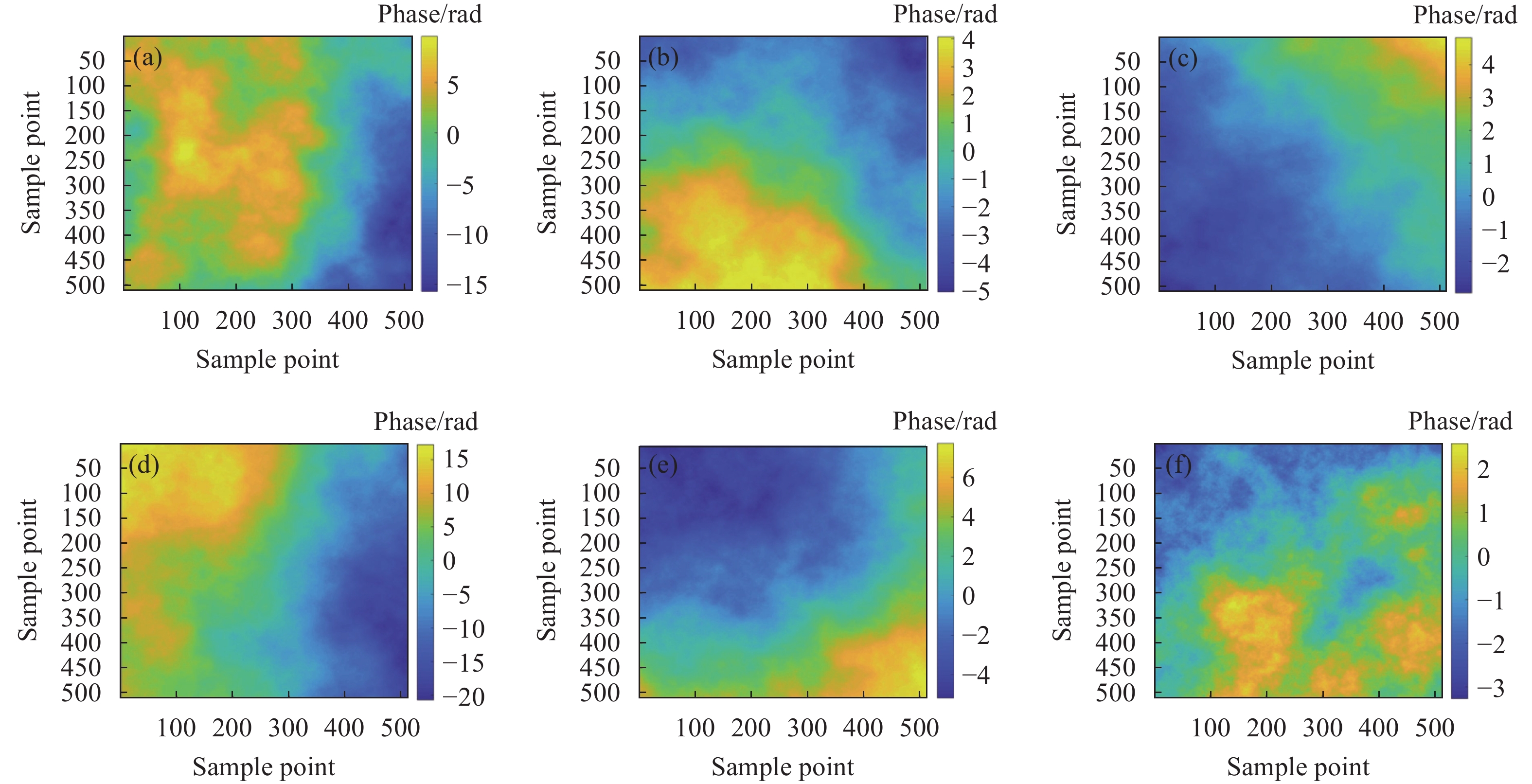
图8和图9分别为采用不同的湍流谱模型（Kolmogorov谱与Non-Kolmogorov谱）模拟的3个大气层的相位屏模拟结果，图9是对图8中每一个相位屏进行低频补偿后的结果。观测图9可以发现，与图8相比，补偿后的相位屏更加光滑。对于边界层的相位屏，即图（a）和图（d）的大气扰动基本一致，均为[−6, 6] rad，这是因为Non-Kolmogorov和Kolmogorov的谱指数在这一层都为11/3。对流层图（b）和图（e）的大气扰动相差也不大，最大的区别在于平流层，在Kolmogorov谱中，大气扰动几乎为0，而Non-Kolmogorov谱生成的相位屏相位扰动比较大。

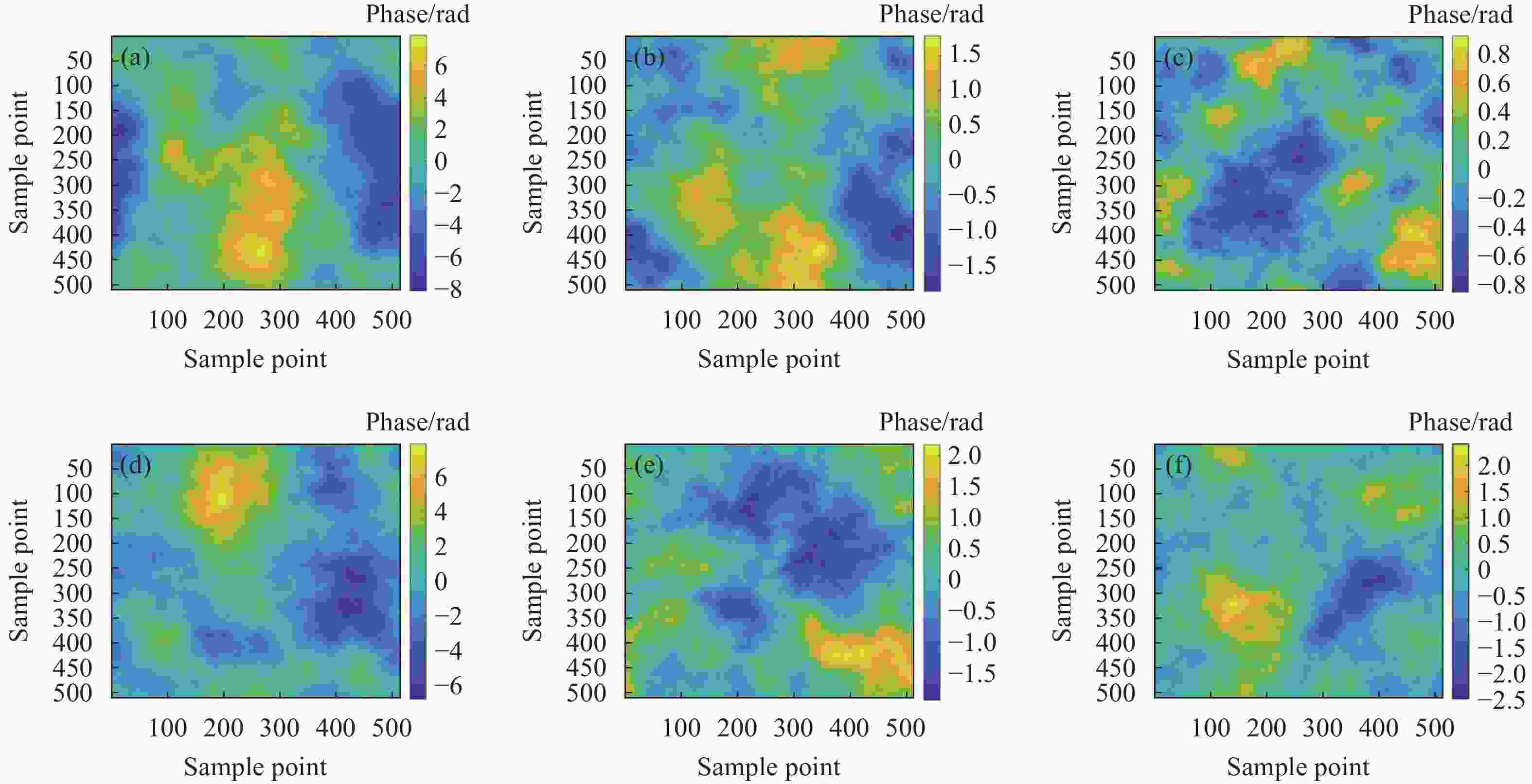
图  8  不同湍流下次谐波补偿前三个大气层对应的相位屏模拟结果。（a）~（c） Kolmogorov； （d）~（f） Non-Kolmogorov

Figure 8.  Simulation results of phase screen simulations corresponding to three atmospheres without harmonic compensation. （a）-（c） Kolmogorov; （d）-（f） Non-Kolmogorov

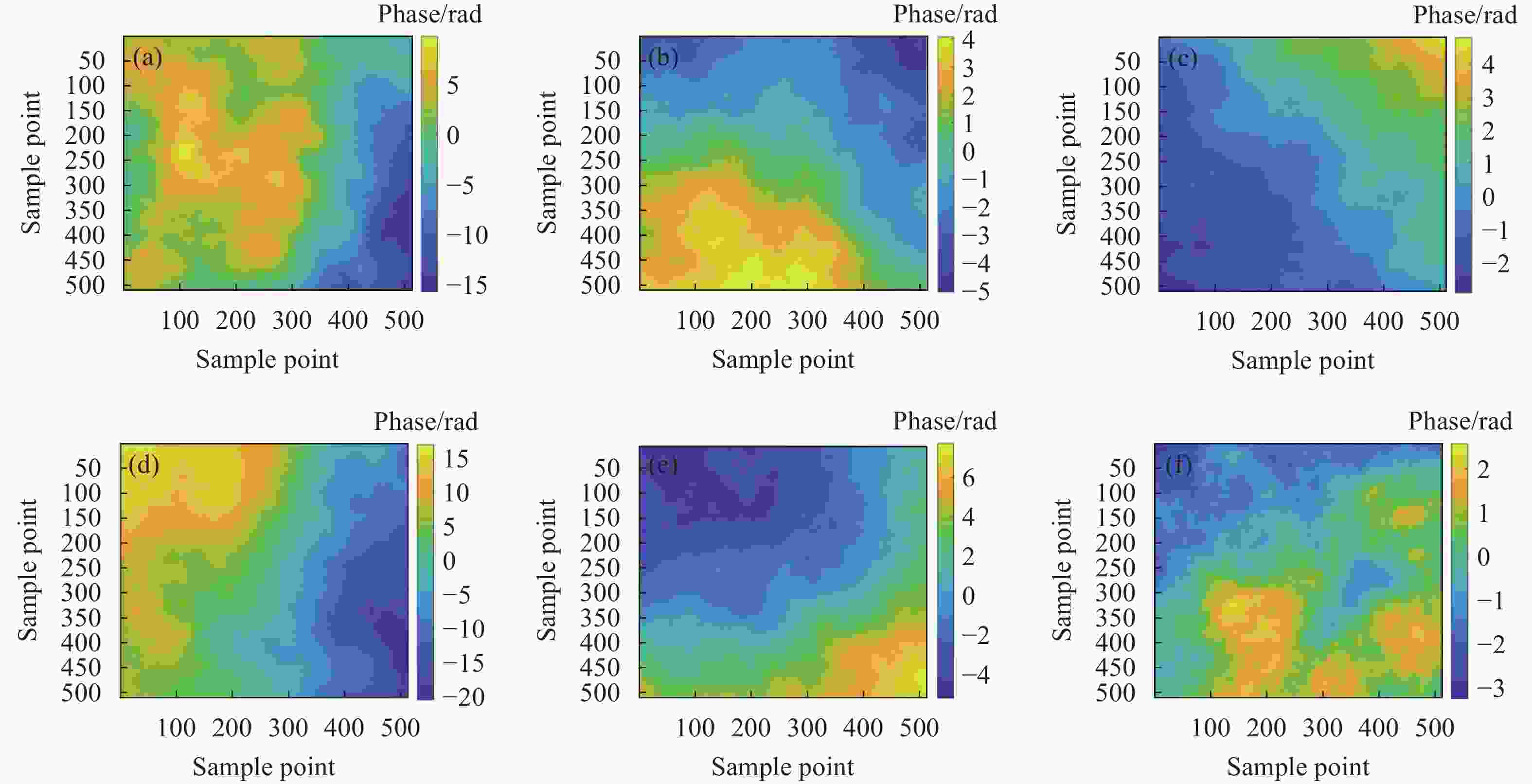
图  9  不同湍流下次谐波补偿后3个大气层对应的相位屏模拟结果。(a)~(c) Kolmogorov；(d)~(f) Non-Kolmogorov

Figure 9.  Simulation results of phase screen simulations corresponding to three atmospheres with harmonic compensation. (a)-(c) Kolmogorov; (d)-(f) Non-Kolmogorov

为了保证湍流模拟的可靠性，图10计算了图8和图9中对应的相位屏补偿前后的相位结构函数与理论值的比较曲线，仿真结果表明，经过次谐波补偿，相位屏均得到了很好的改善，补偿后的相位屏结构函数与理论值更加接近。

图  10  相位结构函数比较

Figure 10.  Comparison of phase structure functions in turbulence simulation

图11是高斯光束分别在Kolmogorov谱和Non-Kolmogorov谱下的传输仿真结果。图中，从左到右分别对应边界层2 km处，对流层10 km处以及平流层20 km处的二维光幅度轮廓分布，图(a)~(c)为Kolmogorov湍流下的传输结果，图(d)~(f)为Non-Kolmogorov湍流下的传输结果。可以发现，无论是Kolmogorov谱还是Non-Kolmogorov谱，在传输过程中，光束中心辐度都会随着传输距离的增加逐渐减小，光束的轮廓也越来越大，即光束扩展现象。在相同的仿真条件下，与谱指数固定不变的Kolmogorov谱相比，当谱指数随传输距离变化时，湍流对传输光的影响更明显，主要体现在更大的光幅度衰减以及更明显的光束扩展。不过，在文中的激光传输数值仿真中，由于参数设置的原因，所以整体高斯光束幅值的改变很小。为了进一步分析非kolmogorov湍流以及Kolmogorov湍流在非均匀的地星链路上对相干光束相干性的影响，图12根据公式（20）绘制了Kolmogorov与Non-Kolmogorov谱下输出光束的相干度在横向距离$r$上的变化。结果表明，在靠近光轴中心的位置，Non-Kolmogorov的相干度要比Kolmogorov谱大，而随着$r$值的增加，NK谱下的光束相干度要比K谱小很多，说明谱指数的动态变化对传输光束的相干性产生了影响。

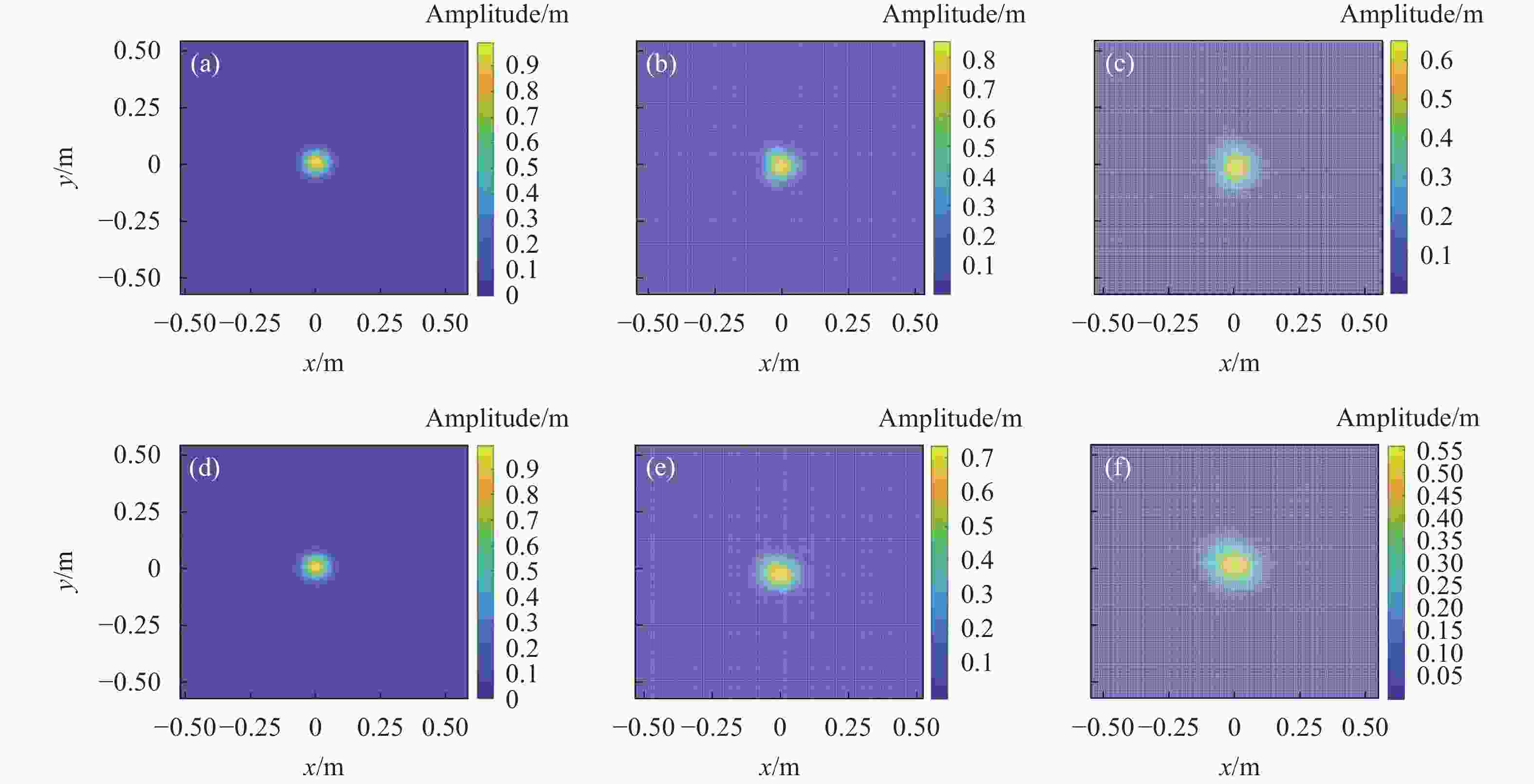
图  11  传输路径上的辐度轮廓变化。(a)~(c) Kolmogorov； (d)~(f) Non-Kolmogorov

Figure 11.  The amplitude profile of the transmitting beam at waist spot. (a)-(c) Kolmogorov; (d)-(f) Non-Kolmogorov

图  12  观测面处的互相干因子

Figure 12.  Mutual coherence factors at the observation plane

针对地星湍流路径不均匀、激光束传输距离远的特点，文中基于分步传输算法以及数值仿真的约束条件，提出了地星3层传输仿真模型，该模型是将湍流路径分成了3层，每一层的湍流依据大气湍流特性采用谱指数不同的谱描述。计算并对比了传统的Kolmogorov谱下相位屏为2层、3层、6层、11层以及21层下观测面光场的互相干因子，并将其与理论值比较，验证了3层传输模型的可行性，在保证了仿真精度的同时，提高了计算机仿真的效率。基于提出的3层传输模型，模拟了传统的Kolmogorov谱与谱指数随高度变化的Non-Kolmogorov谱下高斯光束的传输过程，比较了二者在平均光辐度以及观测面相干性的变化。结果表明，在相同的大气条件下，近地面区域的Kolmogorov谱与Non-Kolmogorov谱的结果基本一致，而随着传输距离的增加，地星上行高斯光束在Non-Kolmogorov谱下会产生明显的幅度衰减以及光束扩展，并且观测面处光场的相干性下降的更快。文中所建立的仿真模型可以采用较少的相位屏和传输次数来评估复杂大气湍流影响下的地星上行链路光传输特性，为预测卫星光学接收器孔径处预期波前行为提供了便利。