


-
工业技术发展至今,对高精度光电跟踪系统的精度要求越来越高,已经达到微弧度级别[1],但跟踪系统在运行时受到多种干扰,其中摩擦对系统的影响最大[2]。摩擦力矩的干扰导致系统出现低速爬行、稳态误差、粘滞运动等现象[3],使系统的控制精度产生误差,因此需要对摩擦模型进行辨识并使用控制方法进行补偿。
在摩擦模型研究领域国内外许多学者深入研究并得到了许多成果。目前,已知的摩擦模型有库伦摩擦模型、库伦摩擦+粘滞摩擦模型、静摩擦+库伦摩擦+粘滞摩擦模型、Stribeck摩擦模型、Dahl模型、Bristle模型、Bliman and Sorine模型和LuGre模型[4-5]等。对摩擦力矩参数辨识的方法更是层出不穷,如文献[6]将摩擦模型的线性部分与非线性部分分离,使用最小二乘法对实验参数进行辨识;文献[7]使用粒子群算法辨识球型电机三个方向的Stribeck摩擦模型的参数;文献[8]提出一种基于粒子群算法的针对LuGre摩擦参数两步辨识方法,利用Stribeck曲线辨识了四个静态参数,利用滞-滑极限振荡曲线辨识动态参数。
自动控制技术发展至今,对于外部扰动的控制补偿算法不断地涌现,其中由中国科学院韩京清教授提出的自抗扰控制[9]因其原理简单、控制效果优异在工程应用中取得了许多卓越的成果。有许多科研工作者在自抗扰控制的基础上不断进行改进,高志强教授等提出的线性自抗扰以及基于带宽的参数整定方法,减少了工作量,在工程上应用广泛[10]。近年来,不断有研究人员将自抗扰控制技术引用到光电跟踪系统中如:文献[11]设计一种三阶非线性扩张状态观测器光电跟踪系统中,提升了系统的跟踪精度;文献[12]将卡尔曼滤波器与扩张状态观测器相结合,提升了系统的扰动隔离性。
文中根据光电跟踪系统特点选用参数少,能更好反应低速时速度抖动情况的Stribeck摩擦模型,使用最小二乘法与粒子群算法结合对Stribeck模型进行参数辨识并建模,将模型数据与实验数据进行比对,分析辨识结果的准确性。使用扰动分离自抗扰控制算法对辨识得到的摩擦模型进行补偿,将补偿结果与在同样扰动条件下的PID控制结果和经典自抗扰控制结果进行比较证明该控制算法能够提升系统的跟踪精度,降低跟踪误差。
-
光电跟踪系统中转台系统采用位置环,速度环以及电流环控制结构,如图1所示。文中以某型转台为例,其直流力矩电机的运动方程为:
$$ \begin{array}{c}u=R\cdot {I}_{d}+L\cdot \dfrac{{\rm{d}}{I}_{d}}{{\rm{d}}t}+E \end{array} $$ (1) $$ \begin{array}{c}M={K}_{i}\cdot {I}_{d}\end{array} $$ (2) $$ \begin{array}{c}E={K}_{e}\cdot \omega \end{array} $$ (3) $$ \begin{array}{c}J\cdot \dfrac{{\rm{d}}\omega}{{\rm{d}}t}=M-{M}_{f}\end{array} $$ (4) 式中:u为电枢电压;R为电枢电阻;L为电枢电感;Id为电枢电流;E为反向电动势;M为电机的输出力矩;$ {K}_{i} $为力矩系数;Ke为反向电动势系数;ω为转速;Mf为摩擦力矩;J为电机的转动惯量。其模型框图如图2所示。
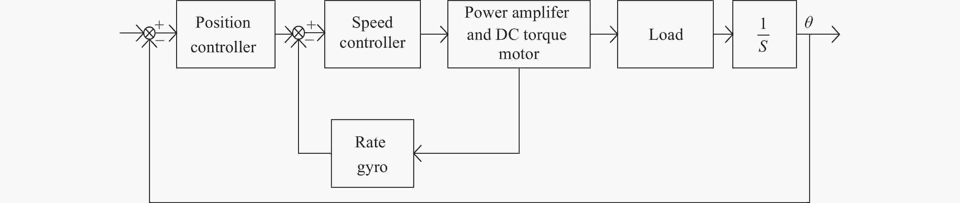
图 1 转台系统结构图
Figure 1. Structure diagram of turntable system

图 2 电机模型图
Figure 2. Motor model diagram
由公式(1)~(4)可以得到系统的运动方程为:
$$ \begin{array}{c}\ddot{\omega }=-\left(\dfrac{R}{L}\right)\cdot \dot{\omega }-\left(\dfrac{{{K}_{i}\cdot K}_{e}}{J\cdot L}\right)\cdot \omega +\left(\dfrac{{K}_{i}}{J\cdot L}\right)\cdot u \end{array} $$ (5) 对公式(5)进行拉氏变换得到其传递函数为:
$$ \begin{array}{c}\phi \left(s\right)=\dfrac{\omega }{u}=\dfrac{1}{{K}_{e}}\cdot \dfrac{1}{\left({T}_{m}s+1\right)\cdot \left({T}_{e}s+1\right)}\end{array} $$ (6) 式中:$ {T}_{m}=\dfrac{J\cdot R}{{K}_{i}\cdot {K}_{e}} $;$ {T}_{e}=\dfrac{L}{R} $。
电机在运动时会受到摩擦力矩的干扰,当电机接收到的电流产生足以克服的最大静摩擦力的力矩时,电机加速转动同时静摩擦力变成库仑摩擦力,此时由于摩擦力矩减小导致电机接收到的电流减小,开始减速。当电流减小到无法克服摩擦力矩的干扰时,电机会停止转动,此时库伦摩擦力变为静摩擦力。由于静摩擦力大于库仑摩擦力,需要增大输入电流。这样反复循环导致了系统在低速时的爬行现象,同样的在低速时摩擦力矩与速度也呈现一定非线性的关系。根据Stribeck摩擦模型电机在运行中速度与摩擦力矩之间的关系为:
$$ \begin{array}{c}{M}_{f}={M}_{c}+\left({M}_{s}-{M}_{c}\right)\cdot {{\rm{e}}}^{[-(\omega /{\omega }_{s}{)}^{2}]}+b \cdot \omega \end{array} $$ (7) 式中:Mc为库伦摩擦力矩;Ms为最大静摩擦力矩;ωs为Stribeck摩擦力矩;b为粘滞摩擦系数;ω为转台角速度,其中Mc、Ms、ωs、b为待辨识的参数。
-
根据公式(7)可知Stribeck摩擦模型在高速转动时,可以近似成线性:
$$ \begin{array}{c}{M}_{f}={M}_{c}+b\cdot \omega \end{array} $$ (8) 将公式(8)与电机的动力学方程结合得到其动力学模型如图3所示。将摩擦模型等效进输入端得到:
$$ \begin{array}{c}J\cdot \ddot{\theta }=\left({i}_{d}-{i}_{f}\right)\cdot {K}_{i}\end{array} $$ (9) 将公式(8)代入公式(9)中得到电机的动力学等效方程(10),其等效图如图4所示。
$$ \begin{array}{c}J\cdot \ddot{\theta }=\left({i}_{d}-{i}_{f}-b\cdot \dfrac{\omega }{{K}_{i}}\right)\cdot {K}_{i}\end{array} $$ (10) 通过向电机输入不同的力矩指令,记录电机的稳态速度,得到速度—力矩关系图,确定Stribeck效应区间。对关系图中高速部分根据公式(10)使用最小二乘法进行拟合即可得到ic与b/Ki的值,即库仑摩擦力与粘滞系数的值。接下来从零开始缓慢增加电流,直到转台开始发生位移,记录下转台在旋转不同角度的启动电流,选取其中最大的电流数值乘以力矩系数可以确定最大静摩擦力矩。获得最大静摩擦力矩、库仑摩擦力矩、粘滞摩擦系数后通过粒子群算法可以拟合出Stribeck速度的数值。

图 3 电机动力学模型图
Figure 3. Motor dynamics model diagram
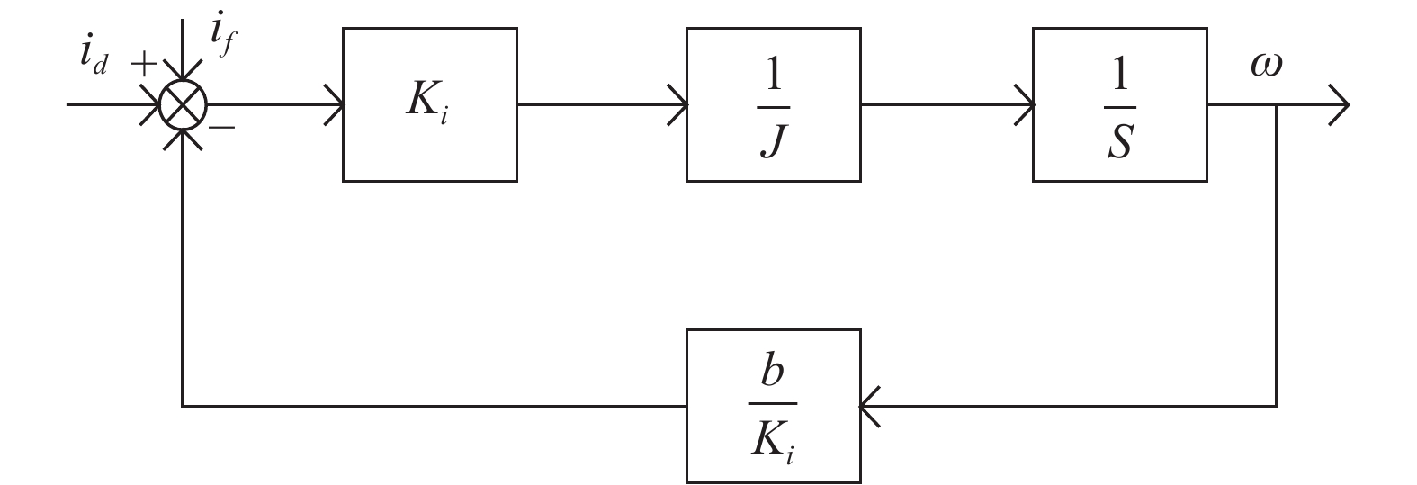
图 4 摩擦模型等效图
Figure 4. Equivalent diagram of friction model
粒子群算法是科学家通过观察、模拟鸟群捕食的过程,演化出的一种进化算法。该算法通过在一个搜索空间中随机生成粒子,每一个粒子都具有随机位置和随机速度,每迭代一轮粒子会产生各自的适应度值,通过筛选每个粒子的适应度值,选择出当前最优适应度粒子,让粒子按照当前最佳适应度粒子的位置与粒子自身最佳适应度位置进行矢量结合确定运动方向,以两个方向速度的加权矢量结合确定运动速度。不断进行迭代从而得到整个过程的最优解。其位置与速度的更新表示为:
$$ \begin{array}{c}{x}_{i}\left(t+1\right)={x}_{i}\left(t\right)+{v}_{i}\left(t+1\right)\end{array} $$ (11) $$ \begin{split} {v}_{i}(t+1)=& p\cdot {v}_{i}\left(t\right)+{c}_{1}\cdot {r}_{1}\cdot \left[{P}_{ib}\right(t)-{x}_{i}(t\left)\right]+\\ & {c}_{2}\cdot {r}_{2}\cdot \left[{P}_{gb}\right(t)-{x}_{i}(t\left)\right] \end{split} $$ (12) 式中:c1和c2分别表示为粒子的个体学习能力和社会共享能力,若c1为零,说明在迭代过程中只有“社会共享”没有“自身学习”,容易出现局部最优的情况;若c2为零,说明在迭代过程中只有“自身学习”没有“社会共享”,导致算法难以收敛。由此可分析出,在c1与c2都不为零的情况下,更易于粒子群算法在搜索范围与收敛速度保持均衡,但c1、c2取值高低同样影响着算法效果,二者取值过低会使粒子在目标区域外徘徊,取值过高会导致粒子越过目标区域,因此一般选取c1、c2的取值范围为[0, 4]之间,文中取c1=c2=2;r1和r2分别为两个[0,1]之间的随机数;Pib、Pgb分别为自身最优适应度值与当前群体的最优适应度值;xi(t)为第t时刻粒子的位置;vi(t)为第t时刻粒子的速度;则xi(t+1)、vi(t+1)为第t+1时刻粒子的位置与速度;p为粒子的惯性因子是一个非负数,其值大小决定着粒子全局寻优能力与局部寻优能力的强弱,数值大代表着全局寻优能力强,局部寻优能力弱;数值小代表着全局寻优能力弱,局部寻优能力强。所以动态的p值较静态的p值相比会得到更好的寻优结果,目前采用较多的是线性递减权值策略[13-14],pmax取0.9,pmin取0.1,G为最大迭代次数,其公式为:
$$ \begin{array}{c}p={p}_{\min}+\dfrac{t\cdot ({p}_{\max}-{p}_{\min})}{G}\end{array} $$ (13) 辨识过程中产生的误差为:
$$ \begin{array}{c}\{{\varepsilon }_{i}{\}}_{i=1}^{N}=\{{\sigma }_{i}{\}}_{i=1}^{N}-\{\stackrel{~}{\sigma }{\}}_{i=1}^{N},\left(i=\mathrm{1,2},\cdots ,N\right) \end{array} $$ (14) 式中:$ \{{\sigma }_{i}{\}}_{i=1}^{N} $为测量得到的力矩数据;$ \{\stackrel{~}{\sigma }{\}}_{i=1}^{N} $为拟合得到的力矩数据。则其个体适应度函数为:
$$ \begin{array}{c}f=\left({\displaystyle\sum }_{i=1}^{N}{\varepsilon }_{i}^{2}\right)^{-1}\end{array} $$ (15) 粒子群算法的具体过程如下:
1) 在一定范围内随机生成一定数量的粒子,确定它们的初始速度与位置,确定辨识次数;
2)对每个随机生成粒子的适应度值进行筛选并更新最佳个体适应度值与最佳群体适应度值;
3)让粒子按照已更新的最佳个体适应度值与最佳群体适应度值更新每个粒子的位置与速度,形成新的粒子群;
4) 达到最大更迭次数后输出最佳群体适应度值对应的粒子作为最优解。
-
扰动分离思想是将系统扰动项从系统中分离,单独作为扩张状态进行补偿,从而可以减少状态观测器的观测负担,并且对原系统的控制器进行复用。
文中提到的扰动为摩擦模型对转台的扰动,根据图2可知摩擦模型对转台的影响公式表示为:
$$ \begin{array}{c}M= \dfrac{(u-E)\cdot {K}_{i}}{(LS+R)}={M}_{f}+JS\cdot \omega \end{array} $$ (16) 令$ G\left(S\right)={K}_{i}/(LS+R $)将公式(16)与公式(3)联立得到:
$$ \begin{array}{c}\omega = \dfrac{G\cdot (u-{M}_{f}/G)}{(JS+{K}_{e}\cdot G)}\end{array} $$ (17) 由此可知,外部摩擦扰动可等效成一个扰动电压ud,令$ {u}_{d}=-{M}_{f}/G $。取x1=$ \omega $, x2=$ \dot{\omega } $,并将等效扰动ud加入到系统的状态空间方程中得到扩张状态空间方程为:
$$ \begin{array}{c}\left\{\begin{array}{c}{\dot{x}}_{1}={x}_{2}\\ {\dot{x}}_{2}=-\left(\dfrac{{{K}_{i}\cdot K}_{e}}{J\cdot L}\right)\cdot {x}_{1}-\left(\dfrac{R}{L}\right)\cdot {x}_{2}+{x}_{3}+\left(\dfrac{{K}_{i}}{J\cdot L}\right)\cdot \left(u+{u}_{d}\right)\\ {\dot{x}}_{3}=h\end{array}\right.\end{array} $$ (18) 式中:x3为被等效扰动项。根据系统的扩张状态空间方程设计的扩张状态观测器为:
$$ \begin{array}{c}\left\{\begin{array}{c}\begin{array}{c}{\dot{z}}_{1}={z}_{2}+{l}_{1}\cdot {e}_{1}\\ {\dot{z}}_{2}=-\left(\dfrac{{K}_{i}\cdot {K}_{e}}{J\cdot L}\right)\cdot {z}_{1}-\left(\dfrac{R}{L}\right)\cdot {z}_{2}+{z}_{3}+\left(\dfrac{{K}_{i}}{J\cdot L}\right)\cdot u+{l}_{2}\cdot {e}_{1}\\ {\dot{z}}_{3}={l}_{3}\cdot {e}_{1}\end{array}\\ {e}_{1}=y-{z}_{1}\end{array}\right.\end{array} $$ (19) 式中:z1、 z2、z3为公式(18)中状态量x1、x2、 x3的估计值;l1、l2、l3为待设计的误差反馈增益。系统的观测误差为:
$$ \begin{array}{c}\left\{\begin{array}{c}{\dot{e}}_{1}={e}_{2}-{l}_{1}\cdot {e}_{1}\\ {\dot{e}}_{2}=-\left(\dfrac{{{K}_{i}\cdot K}_{e}}{J\cdot L}\right)\cdot {e}_{1}-\left(\dfrac{R}{L}\right)\cdot {e}_{2}+{e}_{3}-{l}_{2}\cdot {e}_{1}\\ {\dot{e}}_{3}=h-{l}_{3}\cdot {e}_{1}\end{array}\right.\end{array} $$ (20) 根据带宽法将特征方程的根配置到−ω0处,让误差反馈增益系数按照公式(21)配置,可保证扩张状态观测器保持收敛。
$$ \begin{array}{c}\left\{\begin{array}{c}{l}_{1}=3\cdot {\omega }_{0}- \dfrac{R}{L}\\ {l}_{2}=\left({\dfrac{R}{L}}\right)^{2}-\left(3\cdot \dfrac {R}{L}\right)\cdot {\omega }_{0}+3\cdot {{\omega }_{0}}^{2}-\left( {\dfrac{{{K_i} \cdot {K_e}}}{{J \cdot L}}} \right)\\ {l}_{3}={{\omega }_{0}}^{3}\end{array}\right.\end{array} $$ (21) 选取ω0为大于零的适当值可得到:
$$ \begin{array}{c}\left\{\begin{array}{c}\underset{t\to \infty }{lim}{z}_{1}={x}_{1}\\ \underset{t\to \infty }{lim}{z}_{2}={x}_{2}\\ \underset{t\to \infty }{lim}{z}_{3}=f\end{array}\right.\end{array} $$ (22) 该设计避免了原系统的已知信息的浪费并将扰动通过扩张状态观测器观测出来,以便于补偿器更好的消除扰动,提高控制精度。
-
在设计速度环过程中经常使用期望频率法进行矫正,使系统符合预期的频率特性。期望频率法具有性能稳定、实现简单等特点,但在面对复杂的摩擦情况时对系统的控制能力有限,文中使用该方法对通过扰动分离扩张状态观测器得到状态变量的观测值进行补偿。
由公式(22)可知在观测器选取适当带宽时观测量可以近似为其所观测的状态量,根据期望频率法按照典型Ⅱ型系统的期望开环特性对系统的控制器进行设计。已知典型Ⅱ型系统期望开环特性表示为:
$$ \begin{array}{c}{\phi }_{expect}=K\dfrac{\left(({1}/{{T}_{1}})s+1\right)}{{s}^{2}\left(({1}/{{T}_{2}})s+1\right)}\end{array} $$ (23) 式中:转折频率$ {\omega }_{1}={1/T}_{1} $;$ {\omega }_{2}={1/T}_{2} $;$ {1/T}_{1} \leqslant \sqrt{K}\leqslant {1/T}_{2} $。根据公式(6)可以得到系统的控制器如公式(24)所示:
$$ \begin{array}{c}{G}_{c}=\dfrac{{\phi }_{expect}}{\phi }=K{K}_{e}\dfrac{\left(({1}/{{T}_{1}})s+1\right)({T}_{m}s+1)({T}_{e}s+1)}{{s}^{2}\left(({1}/{{T}_{2}})s+1\right)}\end{array} $$ (24) 可将控制器划分为三个部分。
1)增益部分:
$$ \begin{array}{c}{G}_{c}=K{T}_{m}{T}_{e}{K}_{e}\end{array} $$ (25) 2)超前矫正网络:
$$ \begin{array}{c}{G}_{c1}=\dfrac{({1}/{{T}_{1}})s+1}{({1}/{{T}_{2}})s+1}\end{array} $$ (26) 3)滞后矫正网络:
$$ \begin{array}{c}{G}_{c2}=1+\dfrac{1}{{T}_{m}s}\end{array} $$ (27) $$ \begin{array}{c}{G}_{c3}=1+\dfrac{1}{{T}_{e}s}\end{array} $$ (28) 在此基础上,将扩张状态观测器输出的微分量经过PD控制器引入到系统的控制量中,即:
$$ {u}_{c}=G\left(s\right)\cdot \left({r}-{z}_{1}\right)-{k}_{d}\cdot {z}_{2} $$ (29) -
为了复用原系统的经典控制器,需要将上通过扰动分离扩张状态观测器观测得到的系统的扰动进行补偿,并要求补偿后的系统与原系统理论模型相同。设计的补偿器的控制率为:
$$ \begin{array}{c}u={u}_{c}-{z}_{3}/{b}_{c}\end{array} $$ (30) 式中:uc为控制器的输出;u为被控对象的输入。bc可表示为:
$$ \begin{array}{c}{b}_{c}={K}_{i}/(J\cdot L)\end{array} $$ (31) 通过补偿后得到:
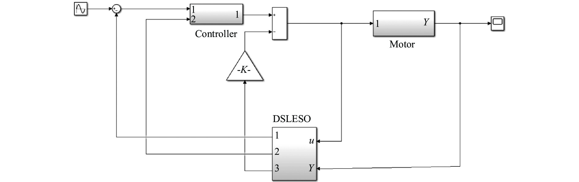
$$ \begin{array}{c}\left\{\begin{array}{c}{\dot{x}}_{1}={x}_{2}\\ {\dot{x}}_{2}=-\left(\dfrac{{{K}_{i}\cdot K}_{e}}{J\cdot L}\right)\cdot {x}_{1}-\left(\dfrac{R}{L}\right)\cdot {x}_{2}+\left(\dfrac{{K}_{i}}{J\cdot L}\right)\cdot \left(u+{u}_{d}\right)\\ {\dot{x}}_{3}=h\end{array}\right.\end{array} $$ (32) 通过公式(32)得到经过补偿的系统模型与原系统的理论模型保持一致。扰动分离自抗扰的控制系统结构图如图5所示。

图 5 扰动分离自抗扰控制系统结构图
Figure 5. Diagram of DSADRC
-
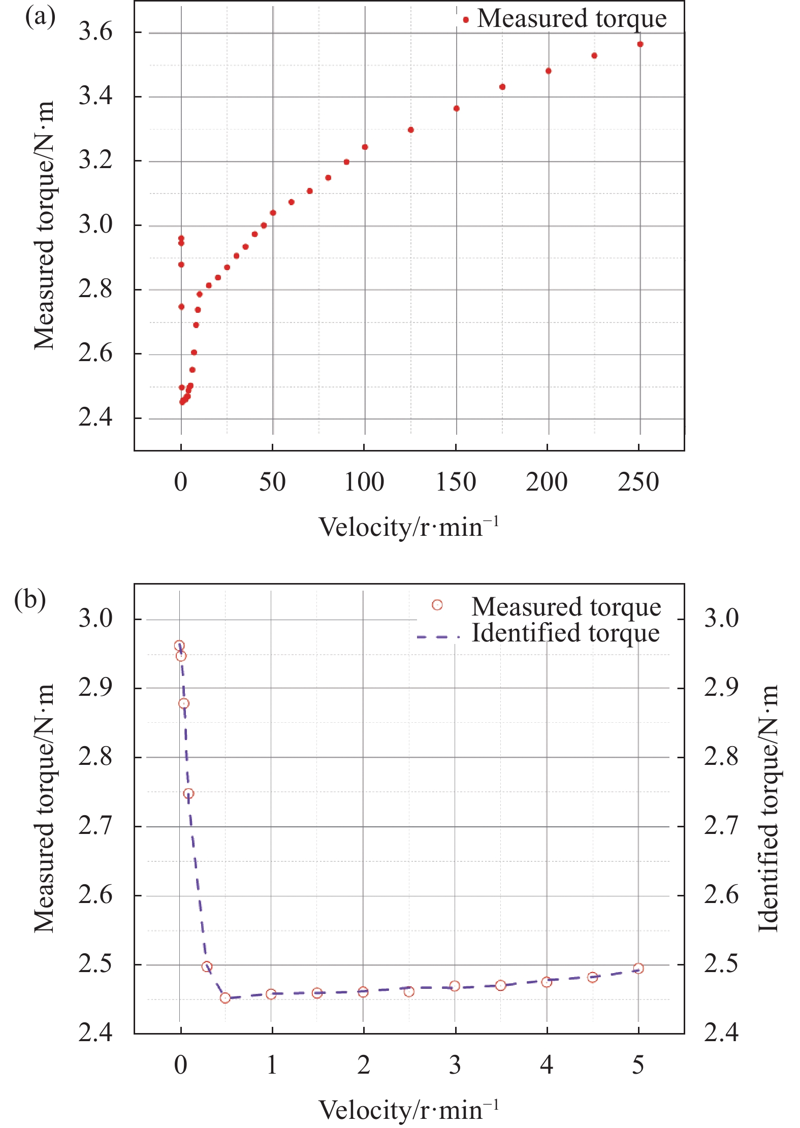
文中选用两轴两框架光电跟踪稳定平台,实验设备图如图6所示,电机参数如表1所示。将转台方位轴按照表2中的转速序列进行实验,在电机速度稳定时,通过Elmo测得电机速度稳定时的电机力矩并绘制速度与力矩对应图如图7(a)所示。选取测量得到的转速-力矩数据的高速部分进行最小二乘法拟合得到库仑摩擦力与粘滞系数,从零开始缓慢增大输入电流直至转台微微旋转,记录此时刻输入的电流值,比较转台在旋转一周后测量得到的电流值,将最大的电流值乘以力矩系数得到最大静摩擦力矩;最后使用粒子群算法对Stribeck速度进行辨识。

图 6 实验设备图
Figure 6. Experimental equipment diagram
表 1 电机参数
Table 1. Motor parameter
Parameter Value L/H 0.0053 R/Ω 1.46 J/kg·m2 5 Ki/N·m·A−1 3.21 Ke/V·r·min−1 0.45 辨识得到摩擦力矩参数见表3。将实验数据与辨识曲线进行对比得到图7(b)。
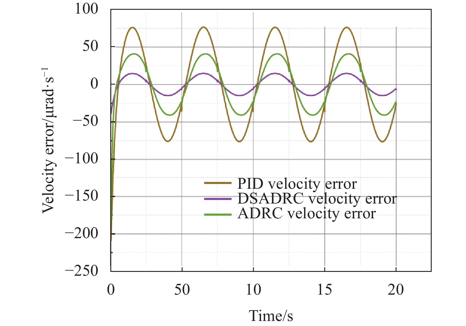
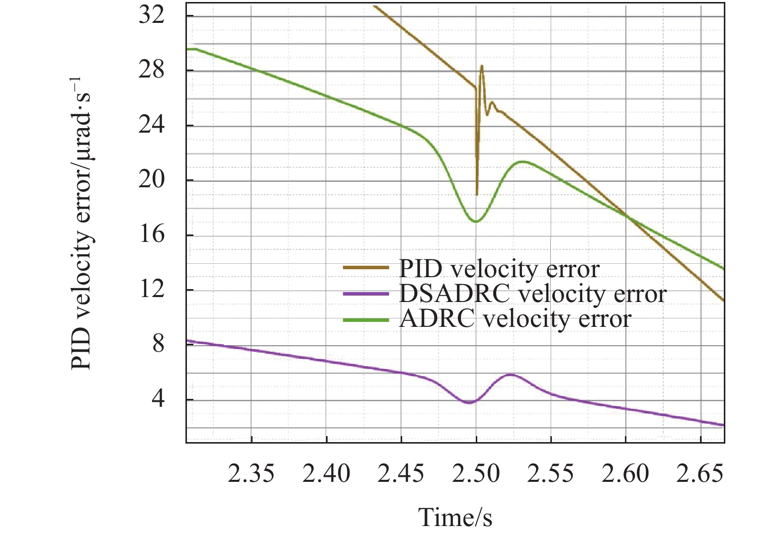
从图7(a)可看出,电机在转速0~5 r/min内出现速度抖动现象。为将该现象充分体现出来,在输入端选择幅值为5°;周期为0.2 Hz的正弦信号作为速度信号。将经过算法辨识得到的摩擦模型加入到转台模型中,分别经过PID控制、自抗扰控制、扰动分离自抗扰控制进行仿真,将仿真结果进行对比。三种控制方法输出速度误差对比图见图8,单边最大速度误差见表4。在图8选取速度为0时刻附近的速度误差数据见图9,通过比较速度抖动幅度判断三种控制方法对摩擦力矩扰动的补偿效果好坏,比较结果见表5。
表 2 转速序列表
Table 2. Speed sequence table
Rotate speed/r·min−1 0.01 0.02 0.05 0.1 0.3 0.5 1 1.5 2 2.5 3 3.5 4 4.5 5 6 7 8 9 10 15 20 25 30 35 40 45 50 60 70 80 90 100 125 150 175 200 225 250 
图 7 (a) 速度-力矩测量数据图;(b) 实验数据与参数辨识对比图
Figure 7. (a) Speed-torque measurement data diagram; (b) Comparison diagram of experimental data and parameter identification
表 3 辨识得到参数表
Table 3. Identified parameter table
Mc/N·m Ms/N·m ωs/r·min−1 b/N·m·r−1·min−2 2.4596 2.9645 0.127 0.0032 
图 8 速度误差对比图
Figure 8. Speed error comparison diagram
表 4 单边最大速度误差表
Table 4. Table of maximum speed error on one side
Control method Maximum speed error on one side/
μrad·s−1PID 75.7817 ADRC 40.9561 DSADRC 16.8814 
图 9 速度为零时刻前后误差图
Figure 9. Error diagram before and after time zero of speed
表 5 受摩擦力矩影响最大速度误差表
Table 5. Table of maximum speed error affected by friction torque
Control method Maximum speed error affected by
friction torque/μrad·s−1PID 6.9096 ADRC 4.6302 DSADRC 1.8249 -
通过最小二乘法与粒子群算法结合辨识得到的摩擦模型与实测数据值的平均误差为3.4%,可以较好地反映电机运行时摩擦模型的真实情况。使用扰动分离自抗扰算法摩擦模型进行补偿,由图8及表4可知,系统经过PID控制的单边最大速度误差为75.7817 μrad·s−1,经过经典自抗扰控制的单边最大速度误差为40.9561 μrad·s−1,经过扰动分离自抗扰的单边最大速度误差为16.8814 μrad·s−1。通过数据比较可以看出,扰动分离自抗扰控制与PID控制相比单边最大速度误差下降了77.72%,扰动分离自抗扰控制与经典自抗扰控制相比单边最大速度误差下降了58.78%,跟踪精度提升。从图9以及表5中可以得到PID控制受摩擦力矩影响最大速度误差为6.9096 μrad·s−1,经典自抗扰控制受摩擦力矩影响最大速度误差为4.6302 μrad·s−1,扰动分离自抗扰控制受摩擦力矩影响最大速度误差为1.8249 μrad·s−1。扰动分离自抗扰控制与传统PID控制相比对摩擦力矩的抑制提升73.59%,与经典自抗扰相比对摩擦力矩的抑制提升60.59%
由此可见,经过扰动分离自抗扰对摩擦模型补偿后系统的跟踪性能有所提升。辨识结果与实测数据之间存在差距的原因:
1)对实验数据高速部分使用最小二乘法进行辨识,忽略Stribeck模型非线性部分对速度的影响,使得对库仑摩擦力矩、粘滞摩擦系数、Stribeck速度的辨识产生误差;
2)润滑脂涂抹不均匀,导致电机转子接触面积不均匀引起了最大静摩擦力矩、摩擦力矩、粘滞摩擦系数发生变化造成误差;
3)电机在进行恒转速实验时,由于电机一直转动产生热量导致其内部零件受热膨胀影响到转子接触面面积发生变化,造成误差。
-
文中针对转台运行中存在Stribeck摩擦力矩进行了最小二乘法与粒子群算法的结合辨识并使用扰动分离自抗扰对其进行补偿。对Stribeck摩擦模型进行分析,使用最小二乘法与粒子群算法分别对Sribeck摩擦模型的低速与高速部分进行辨识,辨识结果与实际值的平均误差为3.4%,可以较好地反应摩擦模型情况。该方法只需通过粒子群算法辨识一个参数,减少辨识工作量。使用扰动分离自抗扰对辨识得到的摩擦模型进行补偿,并将结果与PID控制和经典自抗扰控制得到的结果进行比较。结果证明:扰动分离自抗扰在系统速度单边最大速度误差与PID控制和经典自抗扰控制相比分别下降了77.72%和58.78%;在对摩擦力矩的抑制方面扰动分离自抗扰对比PID控制与传统自抗扰控制分别提升了73.59%和60.59%。综上所述,最小二乘法与粒子群算法结合辨识方法在保证准确率的情况下具有计算量小、节省工作时间的特点,扰动分离自抗扰充分利用了系统的已知信息减少了工作量,同时抑制了摩擦力矩,提升了系统的跟踪精度。
Friction model identification and compensation strategy for photoelectric tracking system
-
摘要: 光电跟踪系统在运行中受到摩擦力矩的影响导致在跟踪过程中产生抖动以及爬坡等现象,严重影响跟踪精度。为提升跟踪精度,结合Stribeck摩擦力矩提出一种最小二乘法与粒子群算法(PSO)结合辨识的方法,建立摩擦模型并使用扰动分离自抗扰(DSADRC)算法进行补偿。首先对转台系统进行建模,分析摩擦对系统的扰动;其次根据Stribeck摩擦模型的特点通过恒转速—力矩实验测得数据,使用最小二乘法与粒子群算法对力矩数据进行辨识,建立起Stribeck模型并将模型等效进系统中;最后使用扰动分离自抗扰控制算法对摩擦模型进行补偿。实验结果表明:最小二乘法与粒子群算法相结合辨识得到的摩擦模型与实测数据之间的平均误差为3.4%,扰动分离自抗扰在单边最大速度误差方面相较于PID控制与经典自抗扰控制分别下降了77.72%和58.78%,在摩擦力矩抑制方面与PID控制和经典自抗扰控制相比分别提升了73.59%和60.59%。
-
关键词:
- 光电跟踪系统 /
- Stribeck摩擦模型 /
- 最小二乘法 /
- 粒子群算法 /
- 扰动分离自抗扰
Abstract:Objective The photoelectric tracking system is affected by frictional torque during operation, resulting in jitter and climbing during the tracking process, which seriously affects the tracking accuracy. For the accurate compensation of frictional torque, this paper proposes a method of least squares method combined with particle swarm optimization algorithm for parameter identification with reference to Stribeck friction model, and uses the disturbance separation active disturbance rejection control (DSADRC) algorithm to compensate the identified friction model. Methods First, the turntable system is modeled to analyze the disturbance of friction on the system. According to the characteristics of Stribeck friction model, the corresponding data were measured by constant speed-torque experiment, and the minimum squares method and particle swarm algorithm were used to identify the moment data, and the Stribeck model was established and added to the system. Then the identified friction model is compensated by using DSADRC. Last, the compensator is designed based on DSADRC. Experimental results show that the average error between the friction model identified by the combination of least squares method and particle swarm algorithm and the measured data is 3.4%. Then PID control, active disturbance rejection control and disturbance separation active disturbance rejection control algorithms are used to control and compensate the friction torque. The results show that the maximum speed error of the disturbance separation active disturbance rejection control is 77.72% and 58.78% (Fig.8, Tab.4) lower than that of the PID control and the active disturbance rejection control respectively. The friction torque suppression of the disturbance separation active disturbance rejection control improves the PID control and the classical ADRC by 73.59% and 60.59% (Fig.9, Tab.5) respectively. The steady state error of the tracking system is reduced, and the tracking performance of the system is improved. Results and Discussions By comparing the results of parameter identification of Stribeck model (Tab.3) with experimental results by using the least squares method and particle swarm algorithm, the average error between the identified friction model and the measured data is 3.4% (Fig.7). And then PID control, active disturbance rejection control and disturbance separation active disturbance rejection control algorithms are used to control and compensate the friction torque. The results show that the single-side maximum speed error of the disturbance separation active disturbance rejection control is 77.72% and 58.78% (Fig.8, Tab.4) lower than that of the PID control and the active disturbance rejection control respectively. The friction torque suppression of the disturbance separation active disturbance rejection control improves the PID control and the ADRC by 73.59% and 60.59% (Fig.9, Tab.5) respectively. Conclusions The parameters of the linear and nonlinear parts of the Stribeck friction model were identified by combining the least squares method and particle swarm algorithm, and the average error between the identification results and the experimental data was 3.4%, which could better reflect the friction model. The friction model is compensated by using disturbance separation ADRC and compared with PID control and ADRC control. The comparison results show that the single-side maximum speed error of the disturbance separation ADRC is 77.72% and 58.78% lower than that of PID control and ADRC control. Compared with PID control and ADRC control on friction torque suppression, the proposed method increases by 73.59% and 60.59% respectively. Through experimental results, it is proved that the disturbance separation self-rejection can not only make full use of the basis of the known information of the system, reduce the waste of information caused by the design, save time, but also reduce the steady-state error of the system, improve the tracking performance of the system, and have certain application value in engineering. -
图 7 (a) 速度-力矩测量数据图;(b) 实验数据与参数辨识对比图
Figure 7. (a) Speed-torque measurement data diagram; (b) Comparison diagram of experimental data and parameter identification
表 1 电机参数
Table 1. Motor parameter
Parameter Value L/H 0.0053 R/Ω 1.46 J/kg·m2 5 Ki/N·m·A−1 3.21 Ke/V·r·min−1 0.45  下载: 导出CSV
表 2 转速序列表
Table 2. Speed sequence table
Rotate speed/r·min−1 0.01 0.02 0.05 0.1 0.3 0.5 1 1.5 2 2.5 3 3.5 4 4.5 5 6 7 8 9 10 15 20 25 30 35 40 45 50 60 70 80 90 100 125 150 175 200 225 250
下载: 导出CSV
表 3 辨识得到参数表
Table 3. Identified parameter table
Mc/N·m Ms/N·m ωs/r·min−1 b/N·m·r−1·min−2 2.4596 2.9645 0.127 0.0032
下载: 导出CSV
表 4 单边最大速度误差表
Table 4. Table of maximum speed error on one side
Control method Maximum speed error on one side/
μrad·s−1PID 75.7817 ADRC 40.9561 DSADRC 16.8814
下载: 导出CSV
表 5 受摩擦力矩影响最大速度误差表
Table 5. Table of maximum speed error affected by friction torque
Control method Maximum speed error affected by
friction torque/μrad·s−1PID 6.9096 ADRC 4.6302 DSADRC 1.8249
下载: 导出CSV
-
[1] 殷宗迪, 董浩, 史文杰, 张锋. 精确模型辨识的光电平台自抗扰控制器[J]. 红外与激光工程, 2017, 46(09): 316-321. Yin Zongdi, Dong Hao, Shi Wenjie, et al. Active disturbance rejection controller of opto-electronic platform based on precision model identification [J]. Infrared and Laser Engineering, 2017, 46(9): 0926001. (in Chinese) [2] 于洋, 张红刚, 高军科, 王建刚. 光电平台角位置信息摩擦观测补偿技术[J]. 红外与激光工程, 2022, 51(05): 309-316. Yu Yang, Zhang Honggang, Gao Junke, et al. Friction observation compensation technology based on angular position information of photoelectric platform [J]. Infrared and Laser Engineering, 2022, 51(5): 20210557. (in Chinese) [3] 翟园林, 王建立, 吴庆林, 孟浩然. 基于Stribeck模型的摩擦补偿控制设计[J]. 计算机测量与控制, 2013, 21(03): 629-631+670. doi: 10.3969/j.issn.1671-4598.2013.03.025 Zhai Yuanlin, Wang Jiangli, Wu Qinglin, et al. Friction compensation control system design based on stribeck model [J]. Computer Measurement & Control, 2013, 21(3): 629-631,670. (in Chinese) doi: 10.3969/j.issn.1671-4598.2013.03.025 [4] Wang Feiyue, Zhang Huaguang, Liu Derong. Adaptive dynamic programming: An introduction [J]. IEEE Comp Int Mag, 2009, 4(2): 39-47. doi: 10.1109/MCI.2009.932261 [5] 刘丽兰, 刘宏昭, 吴子英, 王忠民. 机械系统中摩擦模型的研究进展[J]. 力学进展, 2008(02): 201-213. doi: 10.3321/j.issn:1000-0992.2008.02.006 Liu Lilan, Liu Hongzhao,Wu Ziying, et al. An overview of friction models in mechanical systems [J]. Advances in Mechanics, 2008(2): 201-213. (in Chinese) doi: 10.3321/j.issn:1000-0992.2008.02.006 [6] 曾德豪. 模型辨识技术在机电伺服系统中的应用[D]. 华南理工大学, 2020. Zeng Dehao. Aplication of model identification technology in lectromechanical servo system[D]. Guangzhou: South China University of Technology, 2020. (in Chinese) [7] 李国丽, 李浩霖, 王群京, 琚斌, 文彦. 永磁球形电机Stribeck摩擦模型参数辨识[J]. 电机与控制学报, 2022, 26(04): 121-130. Li Guoli, Li Haolin, Wang Qunjing, et al. Stribeck friction model parameter identification for a permanent-magnet spherical motor [J]. Electric Machines and Control, 2022, 26(4): 121-130. (in Chinese) [8] 张文静, 赵先章, 台宪青. 基于粒子群算法的火炮伺服系统摩擦参数辨识[J]. 清华大学学报(自然科学版), 2007(S2): 1717-1720. doi: 10.3321/j.issn:1000-0054.2007.z2.001 Zhang Wenjing, Zhao Xianzhang, Tai Xianqing. Parameter identification of gun servo friction model based on the particle swarm algorithm [J]. Journal of Tsinghua University(Science and Technology), 2007(S2): 1717-1720. (in Chinese) doi: 10.3321/j.issn:1000-0054.2007.z2.001 [9] 韩京清. 自抗扰控制器及其应用[J]. 控制与决策, 1998, 13(1): 19-23. doi: 10.3321/j.issn:1001-0920.1998.01.005 Han Jingqing. Auto-disturbances-rejection controller and its applications [J]. Control and Decision, 1998, 13(1): 19-23. (in Chinese) doi: 10.3321/j.issn:1001-0920.1998.01.005 [10] 张越杰, 张鹏, 冉承平, 张新勇. 扰动分离自抗扰控制在光电稳定平台上的应用[J]. 红外与激光工程, 2021, 50(10): 244-252. Zhang Yuejie, Zhang Peng, Ran Chengping, et al. Application of a disturbance separation active disturbance rejection control in photoelectric stabilized platform [J]. Infrared and Laser Engineering, 2021, 50(10): 20210068. (in Chinese) [11] 王婉婷, 郭劲, 姜振华, 王挺峰. 光电跟踪自抗扰控制技术研究[J]. 红外与激光工程, 2017, 46(02): 211-218. Wang Wanting, Guo Jin, Jiang Zhenhua, et al. Study on photoelectric tracking system based on ADRC [J]. Infrared and Laser Engineering, 2017, 46(2): 0217003. (in Chinese) [12] 方宇超, 李梦雪, 车英. 基于自抗扰控制的光电平台视轴稳定技术研究[J]. 红外与激光工程, 2018, 47(03): 234-242. Fang Yuchao, Li Mengxue, Che Ying. Study on ADRC based boresight stabilized technology of photoelectric platform [J]. Infrared and Laser Engineering, 2018, 47(3): 0317005. (in Chinese) [13] Shi Y, Eberhart R C. Parameter selection in particle swarm optimization[C]//International conference on evolutionary programming. Berlin, Heidelberg: Springer, 1998: 591-600. [14] Zhang W, Ma D, Wei J, et al. A parameter selection strategy for particle swarm optimization based on particle positions [J]. Expert Systems with Applications, 2014, 41(7): 3576-3584. doi: 10.1016/j.eswa.2013.10.061 -

 点击查看大图

计量
- 文章访问数: 96
- HTML全文浏览量: 3
- PDF下载量: 26
- 被引次数: 0

