


 下载:
下载:


-
在众多数学、物理及工程技术中,物理量随时间或空间位置的动态变化过程可以用微分方程来描述和表示,例如拉普拉斯(Laplace)方程以及泊松(Passion)方程在场问题中的应用,博格斯方程(Burgers’ equation)在流体力学、非线性声学以及交通流等领域的应用,纳维-斯托克斯方程(Navier-Stokes equations)在流体力学中的应用,反应-扩散方程(reaction-diffusion equations)在化学扩散、类波传输过程中的应用,麦克斯韦方程(Maxwell equations)在电磁场问题中的应用。
在过去很长一段时间内,微分方程大都是通过数值方法进行求解。大部分数值方法是基于差分、微元的思想,对计算域进行网格离散,随后通过迭代的方式来获得微分方程的近似解,如有限差分法(FDM)、时域有限差分法(FDTD)、有限元法(FEM)、谱方法(SM)等。目前,数值方法的研究已经十分成熟,被广泛用于解决各类微分方程,多种知名仿真软件的建模基础都是数值方法,如Comsol、Lumerical FDTD以及VPI photonics等。然而,数值方法面临的问题主要是:在复杂场景下(如高非线性、大尺度、高维度等),为了获得稳定、精确的结果,需要对网格进行更精细的划分,且迭代次数与所求场景的尺度成正比,随着场景复杂性的增加,计算量呈指数增长,从而消耗大量计算资源与运算时间;数值方法所消耗的计算资源与时间是不可承受的,这些问题目前依然没有合理的解决方法[1-2]。
自深度学习快速发展以来,大量的研究利用数据驱动方式有监督地训练神经网络,得到输入到输出的映射,间接地求解描述这些问题的微分方程,并且在训练完成后神经网络的预测速度远快于数值方法的求解[3-4]。然而,数据驱动方法的泛化性较差,严重依赖训练数据的多样性与有效性,难以灵活表征动态过程,不能保证在训练数据集所代表的样本空间之外的预测结果的准确性;并且训练过程没有充分考虑已有数学方法及物理理论作为支撑,是一个缺乏可解释性的“黑盒”模型,因此并不能真正替代数值方法。
近几年,在计算物理领域提出了一种具有变革意义的利用神经网络直接求解微分方程的方案——物理信息神经网络(physics-informed neural network, PINN)[5],引起了广泛的关注。与广泛研究的利用数据驱动的方法不同, PINN将取自预设计算域内的微分方程的自变量坐标(一般为时间、空间坐标)作为神经网络的输入,方程的因变量作为输出,随后利用自动微分(automatic differentiation, AD)框架计算方程因变量相对于自变量的各阶导数,构成微分方程,最终将方程以及对应定解条件(一般包括初始条件、边界条件)嵌入到神经网络的损失函数中,通过迭代训练,对网络参数进行优化,使损失函数逐渐趋近于零,同时网络输出也逐渐趋近于方程的真实解,将求解方程的过程巧妙地转换为优化损失函数的过程。在训练过程(即求解过程)中,除去定解条件之外,PINN无需任何标签数据,本质上属于无监督的过程。训练完毕的PINN拟合了微分方程在定解条件下的解函数,本质上是利用了具备数学物理可解释性的神经网络替代了传统数值方法中各个有限元的偏置函数,使训练的物理意义大大增强。
PINN因其强大的求解微分方程的能力,已经在在求解流体动力学、空气动力学以及热力等领域中的微分方程相关的问题中得到成功验证[6–8]。在光纤中,PINN还展示了其在求解非线性薛定谔方程的有效表征能力,并准确地模拟了光纤中波形的演化[9-12]。这些案例充分说明了PINN对求解微分方程相关问题的强大能力及其应用场景的多样性、普适性。
文中着眼于光纤非线性的建模,先后呈现了利用PINN求解:1)描述光信号在光纤中传输受损耗、色散以及非线性等多种物理效应影响而发生演化现象的非线性薛定谔方程(nonlinear Schrödinger equation,NLSE);2)描述光纤中受激拉曼散射导致功率转移的受激拉曼散射(stimulated Raman scattering,SRS)常微分方程;3)描述光模场在结构非均匀光纤中的分布与传输的傍轴亥姆霍兹方程(paraxial Helmholtz equation,PHE)的具体实施方案与结果,并与数值方法进行对比分析,结果表明PINN能够很好地表征三种场景下的动态过程。
-
物理系统的动态过程通常可以用由时间导数、空间导数和非线性项组成的微分方程(differential equation,DE)进行数学表示,微分方程的一般形式可以表述为:
$$ {h}_{t}\left(x,t\right)+N\left[h;\theta \right]=0,\;\;\;x\in \varOmega ,t\in \left[0,T\right] $$ (1) 式中:h为微分方程的潜在解; ht为h的时间导数;N[-:θ]为包括空间导数以及非线性项在内的非线性算子;θ表示每一项的参数;Ω表示求解域;T表示描述问题的时间尺度。
如图1所示,PINN的基本结构包括:神经网络(neural network, NN)、导数计算、微分方程计算以及最小化损失函数四个部分。神经网络分别以微分方程的自变量(x, t)和因变量h作为输入和输出,对于神经网络的输出,采用自动微分 [13]来计算其各导数,进而加和构成完整的微分方程。数值方法依据离散网格上相邻的点计算差分,进而构成差分方程来近似代替微分方程,而在求处于边界上的点的差分时,差分的计算需要用到在计算域之外的点,但域外的点对应的物理量是不可知的,故在求边界点的导数时,必须用适当的边界条件。选择合适的边界条件及参数是至关重要的,若选择不当,则在边界上会引入反射,对计算域内的计算造成误差;而PINN是一种不依赖于网格的方法,可以在求解域内随机采样,利用AD对这些随机采样点对应的潜在解快速地计算导数,不会产生截断误差。需要说明的是,在计算微分方程的过程中,只用到了这些随机采样点的坐标,因此计算微分方程的过程实际上是无监督的。在网络训练过程中,PINN仅需少量的物理约束数据(初始条件或者边界条件)作为定解条件来使网络收敛到该条件下的真实解,而无需采集其他数据,因此PINN本质上属于知识驱动方法,大大减小了对于数据的依赖。损失(Loss)函数包括微分方程损失$ Lo s {s}_{DE} $及物理约束数据损失$ Lo s {s}_{{h}_{0}} $,表达式如下:

图 1 PINN的基本结构:由神经网络、导数计算、微分方程计算和最小化损失函数四个部分组成
Figure 1. The basic structure of PINN consists of four parts: neural network, derivative calculation, partial differential equation calculation, and minimization loss function
$$\begin{split} Lo s s=& M S {E}_{{{{D}}}{{{E}}}}+M S {E}_{{{{{h}}}}_{0}} =\\ & \dfrac{1}{{N}_{r}}\sum _{i=1}^{{N}_{r}}|{h}_{t}+N(h;\theta ){\left.\right|}^{2}+\\ & \dfrac{1}{{N}_{0}}\sum _{i=1}^{{N}_{0}}\left|{h}_{pred}\right({x}_{i},{t}_{i})-{h}_{0}({x}_{i},{t}_{i}){\left.\right|}^{2} \end{split}$$ (2) 式中:MSE表示均方误差,$ M S {E}_{DE} $用于衡量NN的输出代入到微分方程中的误差,该值越小,说明神经网络的输出越符合微分方程;$ M S {E}_{{h}_{0}} $用于衡量NN在物理约束数据点坐标处所得预测值与物理约束数据点对应真实值之间的差距;Nr表示在计算域内随机采样点的数目;N0表示物理约束数据点的数目。随后利用梯度下降法和反向传播法迭代训练,调整NN的参数,不断优化损失函数使其趋近于零,最终使得NN的输出同时满足物理约束以及微分方程,也即得到了微分方程在定解条件下的解。 这就是说,PINN将求解微分方程的问题巧妙地转化为迭代优化损失函数的过程,从而直接、高效地获得微分方程对应于定解条件下的精确解。
-
在光纤中,非线性是基于光纤的光学器件、光信息处理、光子材料设计和光信号传输的物理基础,极大地促进了光纤激光器、光纤放大器、光纤波导和光纤通信的发展。本节针对:光信号在光纤中传输受损耗、色散以及非线性等多种物理效应影响而演化的现象;光纤中功率因受激拉曼散射而发生功率转移的现象;以及光模场在多种结构光纤中的分布与传输过程等三个光纤非线性过程展开研究,详细介绍了利用PINN分别求解这三个场景控制方程的实施步骤及细节,为衡量PINN的准确性,各个场景的结果均与利用传统数值方法在相同模拟设置下所求的结果相比较,依据均方误差(MSE)为衡量指标,结果表明,PINN在三种光纤非线性场景下,均得到了与数值方法有较高一致性的结果,验证了其求解描述光纤非线性的多个微分方程的能力。
-
光信号在光纤中的传输会受到损耗、各阶色散以及非线性等多种物理效应的影响,导致光脉冲在传输的过程中会产生各种畸变,为了准确表征和解释这些物理效应中蕴含的非线性问题,就必须准确求解公式(3)所示的非线性薛定谔方程(NLSE):
$$ \frac{\partial E}{\partial z}+\frac{\alpha }{2}E+\frac{i}{2}{\beta }_{2}\frac{{\partial }^{2}E}{\partial {t}^{2}}-\frac{1}{6}{\beta }_{3}\frac{{\partial }^{3}E}{\partial {t}^{3}}-i\gamma {\left|E\right|}^{2}E=0 $$ (3) 式中:E(z, t)为光信号的复包络;z, t分别为传输距离和参照系中的时间量度。传播参数α、β2、β3、γ分别反映了信号传输过程中的功率损耗、群速度色散(GVD)、三阶色散(TOD)以及自相位调制(SPM)等效应。一般来说,NLSE没有解析解,通常需要采用公式(4)所示的分步傅里叶法(SSMF)等数值方法近似求解:
$$ E\left(z+h,t\right)\approx {\exp}\left(\frac{h}{2}\widehat{D}\right)\mathrm{\exp}\left({\int }_{z}^{z+h}\widehat{N}\left({z}{{'}}\right){\rm{d}}{z}{{'}}\right){\exp}\left(\dfrac{h}{2}\widehat{D}\right)E\left(z,t\right)$$ (4) 式中:D和N分别为NLSE中的线性项和非线性项。SSFM通过交替计算较小步长h上D和N的近似值不断迭代逼近真实解。但是,对于具有高非线性以及长距离传输等情况,步长h需要划分的更小、更多,SSFM等数值方法的计算复杂度会显著增加,难以满足实际建模需求。
为此建立利用PINN求解NLSE实现光纤信道正向建模的方案,在网络训练过程中,PINN仅需物理约束数据(例如发射信号波形)作为定解条件,无需采集其他数据,在NLSE的协同约束下,就能使网络收敛到该约束条件下NLSE的真实解,因此PINN本质上属于知识驱动方法,大大减小了对于数据的依赖。
由于神经网络只能在实数域进行计算,所以需要对NLSE这样的复数方程,需要首先将其分解成实部方程和虚部方程,具体做法为:将E(z, t)改写为其复包络的形式:E(z, t)=u(z, t)+iv(z, t),其中u(z, t)和v(z, t)分别为E(z, t)的实部和虚部,进而NLSE可以分离为如公式(5)所示的实部方程f(u, v)与虚部方程g(u, v),对应地,NN的输入仍为空间坐标,而NN的输出h变成两个:u和v。
$$ \begin{split} & f\left(u,v\right):{u}_{z}+\frac{\alpha }{2}{u}_{z}-\frac{1}{2}{\beta }_{2}{v}_{tt}-\frac{1}{6}{\beta }_{3}{u}_{ttt}+\left({u}^{2}+{v}^{2}\right)v=0 \\ & g\left(u,v\right):{v}_{z}\text+\frac{\alpha }{2}{v}_{z}+\frac{1}{2}{\beta }_{2}{u}_{tt}-\frac{1}{6}{\beta }_{3}{v}_{ttt}-\left({u}^{2}+{v}^{2}\right)u=0 \end{split} $$ (5) 为了计算实部方程f(u, v)与虚部方程g(u, v),需要在求解域内采集若干个离散点坐标作为PINN的输入,通过计算相应的时间与空间导数得到方程值。将计算的f(u, v)、g(u, v)以及预测的初始脉冲复包络$ {\widehat{E}}_{0} $代入损失函数不断优化。当损失低于一个极小值ε,便可以得到光纤中信号演化的过程。为此,团队经验主义地构建了一个具有四个隐藏层,每个隐藏层包含100个神经元的基于PINN的NLSE求解器,其中采用tanh作为激活函数。在大小为[−24T0, 24T0] × [0, 4LD]的计算域上,依据拉丁随机采样法采取50 000个训练点;另外,在初始脉冲信号的实部和虚部上等距离取256个点-值对,分别作为实部方程和虚部方程的初始条件,其中T0表示脉冲宽度,LD=T02/β2表示色散长度。Adam优化算法在数据拟合问题中的表现良好,然而,对于函数优化问题,由于随机梯度下降优化器的一阶导数提供的梯度不完美,可能会导致收敛性能的逐渐恶化甚至波动,特别是在训练的后期。因此在训练过程中,首先使用Adam优化器训练10 000次,使PINN初步收敛于一个相对准确的解,随后采用源自拟牛顿法的有限BFGS (L-BFGS)优化算法来加速PINN的学习,对结果进行进一步优化。
图2 (a)~(c)展示了采用高斯脉冲在不同物理效应作用下,采用上述方法的建模预测演化结果图和以SSFM在相同设置下求得结果为对比的MSE误差密度图。可以看出,在多种效应共同作用、高阶非线性效应等不同场景中,PINN均很好地模拟出信号的演化结果。为了进一步验证PINN方法的普适性,光孤子以及复杂的波形被作为初始条件进行训练,演化结果分别如图2 (d)、(e)所示,结果同样表现出较高的准确性,验证了PINN通过求解描述信号传输过程中功率损耗、群速度色散、三阶色散以及自相位调制等效应的NLSE,模拟光信号在光纤中传输的能力。

图 2 高斯脉冲在(a) GVD和SPM, (b) TOD和SPM,(c) GVD、SPM和自变等陡多种物理效应作用下的预测演化结果和误差密图;GVD和SPM共同作用下(d)一阶光孤子, (e)二 阶光孤子的预测演化结果和误差密度图
Figure 2. Predicted evolution results and error density of Gaussian pulse under various physical effects such as (a) GVD and SPM; (b) TOD and SPM; (c) GVD, SPM, and self-steepening; Predicted evolution results and error density of (d) first-order optical solitons and (e) second order optical solitons under the effect of GVD and SPM
-
在宽带传输波分复用(WDM)系统中,受激拉曼散射(SRS)将功率从高频通道传输到低频通道,是WDM系统的主要损伤。参数化WDM信号(即用平均功率值代表每一个信道) 的功率传输过程由SRS演化常微分方程组(ODE)来描述:
$$ \frac{\partial {P}_{n}\left(z\right)}{\partial z}=-2\alpha {P}_{n}\left(z\right)+{\sum }_{m=1}^{N}\frac{{g}_{R}\left({\omega }_{m}-{\omega }_{n}\right)}{{A}_{eff}}{P}_{n}\left(z\right){P}_{m}\left(z\right) $$ (6) 式中:z为传输距离;Pn代表第n个信道的功率;α为衰减系数;gR为拉曼增益系数;${\omega }_{n} $为第n个信道的频率;N为总信道数量;Aeff为光纤有效模式面积。此SRS 演化常微分方程组的数值解法包括每跨多步计算方法(Multi Step Per Span, MSPS)等。为验证PINN在WDM系统中的可行性,仿真了C+L-band传输系统,传输带宽从186.1~196.1 THz,信道带宽为100 GHz,C和L band之间有600 GHz的保护间隔,满载共96个信道;对应地,SRS演化方程组共有96个常微分方程(ordinary differential equation,ODE),相对应的PINN有96个输出,对应96个信道功率。PINN的输入为在0~80 km的传播区间内随机采样2 000个点zi,损失函数由初始条件(各信道初始功率) Loss和PDE Loss组成,其中初始条件Loss用于控制当z=0时96信道功率的初始条件。如图3所示,PDE Loss由96个ODE方程组成的损失函数矩阵构成。基于PINN的SRS常微分方程求解算子共有四个隐藏层,每层包括100个神经元,以96个信道的初始发射功率谱作为初始约束条件,首先利用Adam优化器迭代训练10 000次,随后利用L-BFGS对PINN进行加速优化。图4展示了PINN以及数值方法MSPS求得的传输距离从0分别到20 km、40 km、60 km以及80 km的结果图,标注了在每个传输距离下的图线旁标注了两种方法的均方误差大小,PINN与MSPS得到了极其接近的结果,MSE随传输距离的增大略有上升,但总体误差仅在1.8×10⁻³量级以内,验证了PINN模拟因受激拉曼散射而导致光功率转移现象的能力。

图 3 PINN求解SRS常微分演化方程组的DE loss示意图,总信道数目N=96
Figure 3. Schematic diagram of PDE loss for solving SRS ordinary differential evolution equations using PINN, with a total number of channels N=96

图 4 数值方法和PINN在传输距离为20/40/60/80 km的结果图
Figure 4. Results obtained by numerical method and PINN at transmission distance of 20/40/60/80 km
在所构建的网络中,共有3 858 816个乘法器。而分步迭代的数值方法在步长为100 m,传输距离为80 000 m的情况下共有707 788 800个乘法器,是PINN的180倍,表明PINN具有更低的计算复杂度。
-
大多数集成光子器件和光纤光子器件都涉及到光在波导中的传播,通过改变光纤的几何结构来定制光传输可以在光纤输出端省去光学元件,这在遥感、材料加工、内窥镜等领域的微型化光传输具有趣的前景[14-17]。为了充分发挥这些应用的潜力,需要对成型光束在给定光纤中的传播过程和物理特性精确建模。光纤中的模场分布及传输受傍轴亥姆霍兹方程(PHE)控制:
$$ 2j\overline{k}\frac{\partial E}{\partial z}=\frac{{\partial }^{2}E}{\partial {x}^{2}}+\frac{{\partial }^{2}E}{\partial {y}^{2}}+\left[{{k}_{0}}^{2}{n}^{2}-{\overline{k}}^{2}\right]E $$ (7) 式中:$ E $为在慢变场假设下的慢变场强;k0为真空波数;$\overline{k}$为参考波数;n(x, y, z)为光纤的三维折射率分布。在数学上,光纤的结构完全由n确定。通过对n做相应的数学变换,可以表征光纤的不同几何结构。PHE依据不同的折射率分布n可以得到初始输入模场在不同几何结构光纤中的演化过程。由于PHE同样是一个复数方程,所以也需要对PHE进行实虚部分离,如公式(8)所示,PHE的实部和虚部方程:
$$ \begin{split} & f:{u}_{xx}+{u}_{yy}+\left({k}_{0}^{2}{n}^{2}+{\overline{k}}^{2}\right)u+2\overline{k}{v}_{z}=0\\ & g:{v}_{xx}+{v}_{yy}+\left({k}_{0}^{2}{n}^{2}+{\overline{k}}^{2}\right)v-2\overline{k}{u}_{z}=0 \end{split} $$ (8) 基于PINN的PHE求解框架如图5所示,考虑到光纤横截面上的模场分布是一种直观、常用的描述模场演化过程的方法,分别以塞尔函数以及变形贝塞尔函数的线性组合表示的五种最低阶LP模式作为初始条件(IC),分别在不同几何结构的阶跃光纤中展示了利用PINN求得的模场演化的结果。需要说明的是,初始输入模场同样需要进行实虚部分离的处理,分离得到的实部和虚部被分别设置为实部方程和虚部方程的初始条件,在文中验证方案中,在输入模场的实部和虚部上均随机采样N0=10 000个点,分别作为实部方程和虚部方程初始条件;另外,用于求解PHE的PINN包含四个隐藏层,每层包含100个神经元,采用tanh作为激活函数,在(x, y, z)∈[−25 μm, 25 μm]×[−25 μm, 25 μm]×[0, 1000 μm]的三维计算域内,依据拉丁随机采样方法采Nr=200 000个采样点,首先利用Adam优化器迭代训练300 000次,随后利用L-BFGS对PINN进行加速优化。

图 5 基于PINN的PHE求解框架
Figure 5. PINN-based solving scheme
在直阶跃光纤中,芯层和包层的折射率均为定值,芯层折射率ncore略大于包层折射率nclad。在本节的所有验证方案中,物理参数设置为:光波长λ=1.064 nm,光纤参数ncore=1.523、nclad=1.52以及纤芯半径r=12.5 μm。对于直光纤,傍轴亥姆霍兹方程具有解析解(即LP模),形式上可以表述为E=E0$ {{\rm{e}}}^{-j\beta z} $,表明在直光纤中,PHE将沿着传播轴对输入的LP模式在幅度上稳定传播,在相位上周期性传播,也就是说在任意的传播距离处的横截面内,都有着相同的绝对归一化强度。
光纤的拉锥表现为沿着传播方向,光纤的芯层逐渐变细,在数学上以沿着传播方向逐渐缩放折射率剖面的芯层半径来表示[18]:
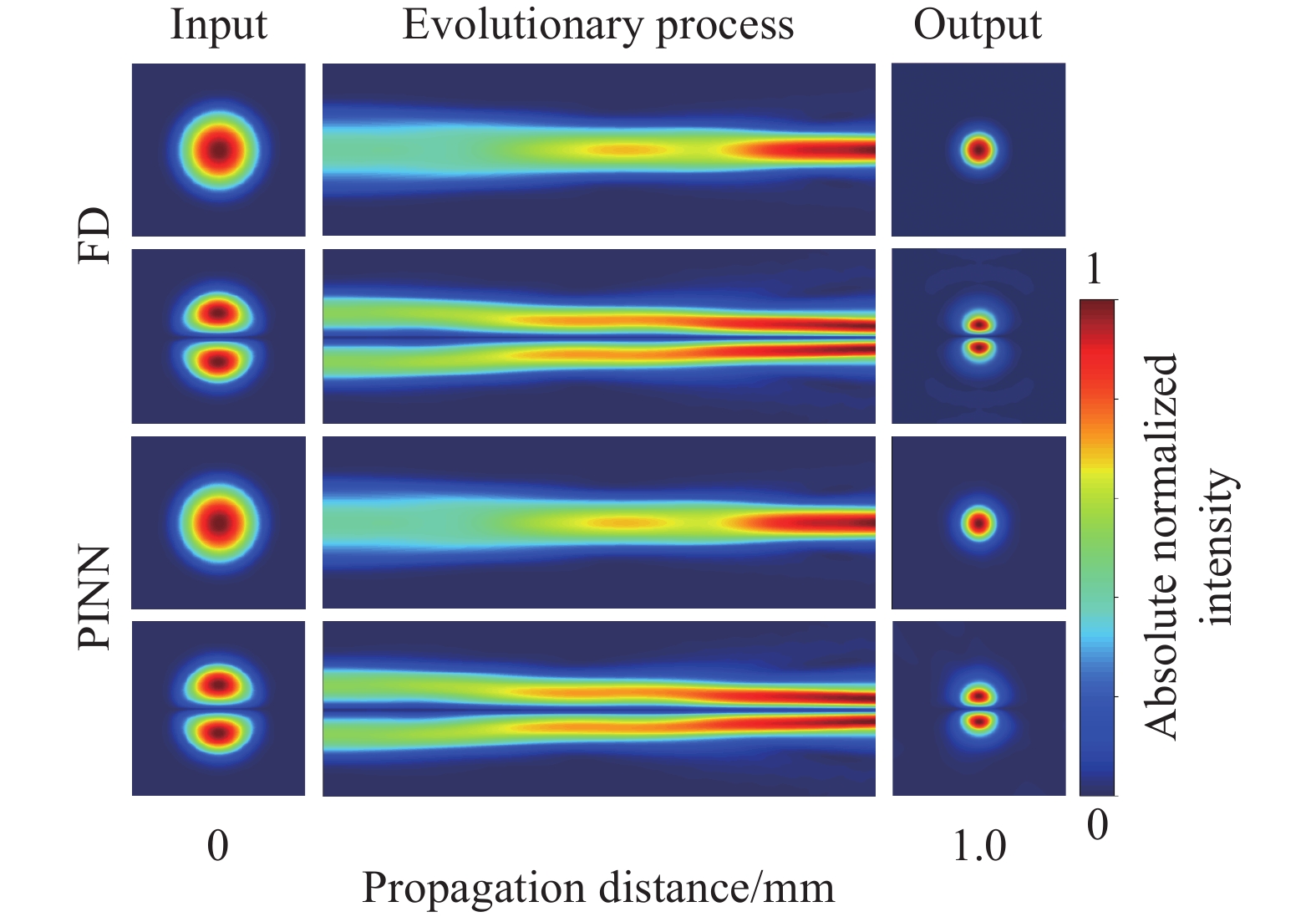
$$ r\left(z\right)=r\left(0\right)\left[1-\left(1-S\right)\frac{z}{{L}_{z}}\right] $$ (9) 式中:r(z)为传播距离z处的芯层半径;S为锥度,定义为光纤末端芯区半径与初始端芯层半径的比;Lz为光纤长度。图6展示了将LP01、LP11o模输入到S=0.37的拉锥光纤中,分别采用有限差分法波束传播法(finite difference beam propagation method, FD-BPM)和PINN求解PHE得到的模场在y-z平面内的演化过程,二者结果有较高的一致性,可以看到随着纤芯半径的收缩,光场模斑逐渐表笑,即模场的功率随着光纤的变细而逐渐汇聚。

图 6 分别以 FD 及 PINN 求解 PHE 得到 LP01、 LP11o模在拉锥光纤中y-z平面内的演化图
Figure 6. Evolution process of LP01 and LP11o modes in the y-z plane of tapered fiber obtained by FD and PINN by solving the PHE
光纤的弯曲效应通过利用保角变换技术[19],将直光纤垂直于传播方向横截面内的折射率分布n(x, y)转换为横截面内坐标的函数来表征,如公式(10)所示:
$$ {n}{{{'}}}\left(x,y\right)=n\left(x,y\right)\left[1-{n}^{2}\left(x,y\right)\frac{x}{2R}{p}_{e}\right]\mathrm{exp}\left(\frac{x}{R}\right) $$ (10) 式中:R为光纤弯曲的曲率半径;pe由泊松比和光弹性张量构成。图7显示了LP01,LP11e,LP11o,LP21e,LP21o五种线偏振模式的模场在弯曲半径R=30 mm,pe=0.3的光纤中不同传播距离处横截面内的模场分布。由于LP模式不是弯曲光纤的导模,模场在传播时会发生模式重叠效应,输入的LP模式相应地会投影到弯曲光纤的各个导模(也即弯曲光纤的正交本征解)上进行干涉传播,从而使模场分布随传播距离而发生演化。

图 7 分别以FD及PINN求解PHE得到五种LP模式在弯曲光纤中不同传播距离处的模斑图
Figure 7. Mode speckle of five LP modes at different propagation distances in bent fibers obtained by FD and PINN by solving the PHE

图 8 以 FD 为对照的利用 PINN 求得五种 LP 模式在三种几何结构光纤中(S: 直; B: 弯曲; T: 拉锥) MSE随传播距离变化曲线
Figure 8. MSE variation curve with propagation distance for five LP modes in three geometric structures of optical fibers by PINN corresponding to FD-BPM
图8展示了在直、拉锥以及弯曲光纤中分别以不同模式作为输入,以FD求得模场数据为参照的横截面内模场MSE随传输距离变化的曲线。总体来看,三种光纤几何结构场景下的MSE均会随着传播距离的增长而有所增长,高阶模式的演化结果相对于低阶模式误差较大;在直光纤的场景中有着较小的误差,误差在10−6量级,拉锥光纤次之,弯曲光纤场景相较于前两者误差相对较大,但总体误差仍在3×10⁻⁴以内,这是因为在将LP模式输入到弯曲光纤中时,PINN对于初始条件的收敛具有一定难度,从而导致在计算域内取得误差相对较大的结果。需要说明的是,PINN在求解PHE时需要经过实虚部分离的过程,神经网络以空间坐标(x, y, z)为输入,以实部方程和虚部方程的解(u, v)为输出,因此PINN不仅能够得到光模场传输与演化各个位置处的幅度信息,也能得到在各个位置处的相位信息,这两个物理量均由(u, v)计算而得,因此以幅度信息的MSE曲线来衡量准确性同样适用于相位信息。该方案验证了PINN通过求解PHE来模拟输入光场在不同几何结构的光纤中传输及演化的能力。图9显示了三种光纤结构场景下,PINN与有限差分方法计算复杂度及归一化运算时间随传播距离的变化,其中,复杂度以乘法器数目为依据。可以看到,有限差分方法的复杂度与场景的选择有关,且其复杂度与纵向网格数目(即迭代次数)成正比,复杂度随传播距离的增加而增加,相应地,运行时间也增加; PINN的计算复杂度与采样点的数目成正比,采样点数目越多,其复杂度相应就越高;虽然PINN的训练需要一定基数采样点数,但是随传播距离的增大,只需略微增加采样点数目,传播距离与采样数目并不呈现出正比关系,因此,在短计算距离下,PINN的复杂度高于有限差分数值方法,而在大规模的长传播距离的场景下,则能体现出PINN低计算复杂度的优势。

图 9 PINN与有限差分方法计算复杂度(a)及运算时间(b)的比较
Figure 9. Comparison of computational complexity (a) and running time (b) between PINN and finite difference method
-
微分方程的求解在众多数学、物理及工程中起着重要作用,文中从求解偏微分方程的数值方法以及基本的利用数据驱动的人工智能算法的背景出发,讨论了两类方法在求解偏微分方程的利弊所在,继而引出了近年来在科学计算领域提出的能够兼顾数学物理定律并且具有可解释性的人工智能算法——物理信息神经网络。物理信息神经网络由于其强大的求解偏微分方程的能力及其普适性,已经在多个领域内的偏微分方程相关的问题中得到成功验证。文中着眼于光纤非线性的建模,先后呈现了物理信息神经网络在求解:1)描述光信号在光纤中传输受损耗、色散以及非线性等多种物理效应影响而演化的非线性薛定谔方程;2)描述光纤中受激拉曼散射导致功率转移的受激拉曼散常微分方程;3)描述光模场在非均匀结构光纤中的分布与传输的傍轴亥姆霍兹方程的能力,物理信息神经网络所得结果与数值方法均有较高的一致性,验证了物理信息神经网络对光纤非线性建模的强大能力。物理信息神经网络备受关注的原因不仅仅在于其正向求解微分方程问题的强大能力;对于系数待定的微分方程,它还能依据少量的观测数据来确定待定系数,进而确定微分方程所描述场景中的未知参数,也即解决逆问题。
传统的科研领域逐步成为人工智能的主战场,人工智能深入到科学研究和技术创新的方方面面。自物理信息神经网络被提出以来,与之相关的研究成果呈爆发式涌现,各类改进及变体算法被不断提出,在加入更多的物理性、研究其训练机理、处理高频问题、噪声问题、大尺度及反向设计等多个方面不断对物理信息神经网络进行完善与改进。具有强大非线性函数学习能力的神经网络被寄希望于建立各种偏微分方程控制下从任意输入空间到任意输出空间的映射关系,也即以数据驱动的方式得到偏微分方程对于物理量的转换算子(operator),与传统的数据驱动方法不同的是,该方法同样可以引入物理引导的思想嵌入偏微分方程,进而构成物理信息神经算子(physics-informed neural operator, PINO),该方法可以准确预测多种定解条件下的解函数,并且在未经训练的定解条下也有较好的预测精度。
目前,人工智能驱动的科学计算社区正在逐步完善,引入物理信息的人工智能算法在未来可能为光纤非线性建模提供一种新思想、新方法、新工具,其可能从根本上为包括光纤非线性建模在内的各个领域在科学计算、设计、建模等方面提供一种可靠的解决方案。
Nonlinear dynamic modeling of fiber optics driven by physics-informed neural network
-
摘要: 近年来,在计算物理领域提出了一种具有变革意义的利用神经网络直接求解微分方程的方案——物理信息神经网络(physics-informed neural network, PINN), 引起了广泛关注, 并且已经在多个领域的微分方程相关的问题中都得到了成功的验证。着眼于光纤非线性的建模,针对光纤中:光信号传输时受损耗、色散以及非线性等多种物理效应影响而发生演化;受激拉曼散射引起的功率转移;光模场在多种几何结构光纤中的分布与传输这三个场景展开研究。在数学上,这三个场景的控制方程分别为:非线性薛定谔方程、受激拉曼散射常微分方程以及傍轴亥姆霍兹方程,文中先后呈现了利用PINN求解这三个方程的具体实施方案及结果,并与数值方法进行对比分析,二者结果显示出较高的一致性, 且PINN具备更低的计算复杂度。PINN作为一种精准、高效的微分方程求解框架,在未来有潜力推进光纤非线性建模的发展。Abstract:
Objective In the field of nonlinear dynamic of fiber optics, various fiber optic effects can be mathematically described by differential equations such as the nonlinear Schrödinger equation (NLSE) that describes the evolution of optical signals due to many physical effects such as loss, dispersion and nonlinearity; Stimulated Raman scattering (SRS) ordinary differential equation describes the power evolution caused by stimulated Raman scattering; And the paraxial Helmholtz equation (PHE) describes the distribution and propagation of optical mode fields in fibers with various geometric structures. For a long time in the past, differential equations, including these three equations, were solved using numerical methods, most of which are based on the idea of difference and microelement, and discretize the computational domain and then obtain the approximate solution of the differential equation through iteration, such as finite difference method (FDM), finite-difference time-domain method (FDTD), finite element method (FEM), spectral method (SM), etc. However, the main problems faced by numerical methods are as follows. In complex scenes (such as high nonlinearity, large scale, high dimension, etc.), in order to obtain stable and accurate results, it is necessary to divide the grid more precisely, and the number of iterations is proportional to the scale of the desired scene. As the complexity of the scene increases, the amount of computation increases Exponential growth, which consumes a lot of computing resources and computing time; The computational resources and time consumed by numerical methods are unbearable, and there is currently no reasonable solution to these problems. Therefore, it is necessary to introduce a new equation solving tool with the properties of efficiency and low complexity to avoid the difficulties faced by numerical methods to meet the needs of accurate modeling of the dynamic process of interest physical quantity in complex scene. In recent years, in the field of computational physics, a revolutionary scheme for directly solving differential equations using neural networks, the physics-informed neural network (PINN), was proposed, which has attracted widespread attention and has been successfully validated in various fields related to differential equations. For the purpose of accurate modeling of nonlinear dynamic of fiber optics, PINNs were employed to solve NLSE, SRS ordinary differential equation and PHE to preliminarily verify PINN's feasibility in the field of fiber optics in this paper. Methods The principle of PINN is firstly elucidated in this paper (Fig.1). Since PINN is real-valued, while the NLSE and PHE are actually complex equations. Thus, when solving these two equations by PINN, it is necessary to first separate the real and imaginary parts of the equation to obtain the real and imaginary part equations (Eq.5, Eq.8, Fig.5). The loss function of SRS ODE is reformed in the form of a matrix due to the coupling effect between different channels (Fig.3). Taking mean square error as accuracy evaluator, the results of NLSE, SRS ODE and PHE obtained by PINN are respectively compared with that of split-step Fourier method (SSFM), multi-step per span (MSPS) method and finite difference beam propagation method (FD-BPM) (Fig.2, Fig.4, Fig.6-8) to verify the feasibility of PINN for the modelling of nonlinear dynamic of fiber optics. Additionally, the computational complexity and running time of PINN and numerical method is quantitatively analyzed (Fig.9). Results and Discussions The feasibility of PINN for solving NLSE is verified in the scenario that considers the effects of group velocity dispersion (GVD), self-phase modulation (SPM) and third order dispersion (TOD) with multiple input signals such as Gaussian pulse, first-order soliton and second-order soliton in the transmission distance of 80 km (Fig.2). The verification scenario of SRS ODE is set to the C+L-band transmission system of a transmission bandwidth from 186.1 THz to 196.1 THz, a channel bandwidth of 100 GHz, and a protection interval of 600 GHz between C and L bands, which has a total of 96 channels under full load (Fig.4). The PHE is solved respectively in step-index fiber in the geometry of straight, bended and tapered with five lowest linear polarization modes employed as fiber inputs (Fig.6-8). The above validation schemes all achieved accuracy results compared to those of numerical methods with low computational complexity and running time (Fig.9). Conclusions As a revolutionary differential equation solving scheme, PINNs are introduced to the modelling of the nonlinear dynamic of fiber optics in this paper. The feasibility of PINN is verified in three typical nonlinear scenarios by solving the NLSE, the SRS ODE and the PHE. At present, the scientific computing community driven by artificial intelligence is gradually improving. Artificial intelligence algorithms that introduce physical information may provide a new idea, method, and tool for nonlinear dynamic modelling of fiber optics in the future, which may fundamentally provide a reliable technique for various fields including modeling of nonlinear dynamic of fiber optics in scientific computing, design, modeling, and other aspects. -
图 1 PINN的基本结构:由神经网络、导数计算、微分方程计算和最小化损失函数四个部分组成
Figure 1. The basic structure of PINN consists of four parts: neural network, derivative calculation, partial differential equation calculation, and minimization loss function
图 2 高斯脉冲在(a) GVD和SPM, (b) TOD和SPM,(c) GVD、SPM和自变等陡多种物理效应作用下的预测演化结果和误差密图;GVD和SPM共同作用下(d)一阶光孤子, (e)二 阶光孤子的预测演化结果和误差密度图
Figure 2. Predicted evolution results and error density of Gaussian pulse under various physical effects such as (a) GVD and SPM; (b) TOD and SPM; (c) GVD, SPM, and self-steepening; Predicted evolution results and error density of (d) first-order optical solitons and (e) second order optical solitons under the effect of GVD and SPM
图 3 PINN求解SRS常微分演化方程组的DE loss示意图,总信道数目N=96
Figure 3. Schematic diagram of PDE loss for solving SRS ordinary differential evolution equations using PINN, with a total number of channels N=96
图 4 数值方法和PINN在传输距离为20/40/60/80 km的结果图
Figure 4. Results obtained by numerical method and PINN at transmission distance of 20/40/60/80 km
图 6 分别以 FD 及 PINN 求解 PHE 得到 LP01、 LP11o模在拉锥光纤中y-z平面内的演化图
Figure 6. Evolution process of LP01 and LP11o modes in the y-z plane of tapered fiber obtained by FD and PINN by solving the PHE
图 7 分别以FD及PINN求解PHE得到五种LP模式在弯曲光纤中不同传播距离处的模斑图
Figure 7. Mode speckle of five LP modes at different propagation distances in bent fibers obtained by FD and PINN by solving the PHE
图 8 以 FD 为对照的利用 PINN 求得五种 LP 模式在三种几何结构光纤中(S: 直; B: 弯曲; T: 拉锥) MSE随传播距离变化曲线
Figure 8. MSE variation curve with propagation distance for five LP modes in three geometric structures of optical fibers by PINN corresponding to FD-BPM
-
[1] Hart J K, Martinez K. Environmental sensor networks: A revolution in the earth system science? [J]. Earth-Science Reviews, 2006, 78(3-4): 177-191. doi: 10.1016/j.earscirev.2006.05.001 [2] Alber M, Tepole A B, Cannon W R , et al. Integrating machine learning and multiscale modeling—perspectives, challenges, and opportunities in the biological, biomedical, and behavioral sciences [J]. NPJ Digital Medicine, 2019, 2(1): 1-11. doi: 10.1038/s41746-019-0193-y [3] Wang D, Song Y, Li J, et al. Data-driven optical fiber channel modeling: a deep learning approach [J]. Journal of Lightwave Technology, 2020, 38(17): 4730-4743. doi: 10.1109/JLT.2020.2993271 [4] Yang H, Niu Z, Xiao S, et al. Fast and accurate optical fiber channel modeling using generative adversarial network [J]. Journal of Lightwave Technology, 2021, 39(5): 1322-1333. doi: 10.1109/JLT.2020.3037905 [5] Raissi M, Perdikaris P, Karniadakis G E. Physics-informed neural networks: A deep learning framework for solving forward and inverse problems involving nonlinear partial differential equations [J]. Journal of Computational Physics, 2019, 378: 686-707. doi: 10.1016/j.jcp.2018.10.045 [6] Jin X, Cai S, Li H, et al. NSFnets (Navier-Stokes flow nets): Physics-informed neural networks for the incompressible Navier-Stokes equations [J]. J Comput Phys, 2021, 426: 109951-109977. doi: 10.1016/j.jcp.2020.109951 [7] Mao Z, Jagtap A D, Karniadakis G E. Physics-informed neural networks for high-speed flows [J]. Comput Method Appl M, 2020, 360: 112789-112804. doi: 10.1016/j.cma.2019.112789 [8] Cai S, Wang Z, Wang S, et al. Physics-informed neural networks for heat transfer problems [J]. ASME J Heat Transfer, 2021, 143(6): 060801-060816. doi: 10.1115/1.4050542 [9] Wang D, Jiang X, Song Y, et al. Applications of physics-informed neural network for optical fiber [J]. Communications Magazine, 2022, 60(9): 32-37. doi: 10.1109/MCOM.001.2100961 [10] Jiang X, Wang D, Fan Q, et al. Solving the nonlinear schrödinger equation in optical fibers using physics-informed neural network[C]//Optical Fiber Communication Conference (OFC) 2021: M3H8. [11] Zang Y, Yu Z, Xu K, et al. Principle-driven fiber transmission model based on PINN neural network [J]. J Light Technol, 2022, 40(2): 404-414. doi: 10.1109/JLT.2021.3139377 [12] Jiang X, Wang D, Fan Q, et al. Physics-informed neural network for nonlinear dynamics in fiber optics [J]. Laser & Photon Rev, 2022, 16(7): 1-15. doi: 10.1002/lpor.202100483 [13] Baydin A G, Pearlmutter B A, Radul A A, et al. Automatic differentiation in machine learning: a survey [J]. J Mach Learn Res, 2201, 8: 18, 1-43. [14] Andresen E R, Sivankutty S, Tsvirkun V, et al. Ultrathin endoscopes based on multicore fibers and adaptive optics: a status review and perspectives [J]. J Biomed Opt, 2016, 21(12): 121506-121524. doi: 10.1117/1.JBO.21.12.121506 [15] Danny Noordegraaf, Peter M W Skovgaard, Martin D Nielsen, et al. Efficient multi-mode to single-mode coupling in a photonic lantern [J]. Opt Expres, 2009, 17: 1988-1994. doi: 10.1364/OE.17.001988 [16] Nick Van de Giesen, Susan C Steele-Dunne, Jop Jansen, et al. Double-ended calibration of fiber-optic raman spectra distributed temperature sensing data [J]. Sensors, 2012, 12(5): 5471-5485. doi: 10.3390/s120505471 [17] Wang P, Brambilla G, Ding M, et al. High-sensitivity, evanescent field refractometric sensor based on a tapered, multimode fiber interference [J]. Opt Lett, 2011, 36: 2233-223. doi: 10.1364/OL.36.002233 [18] Veettikazhy M, Hansen A K, Marti D, et al. BPM-Matlab: an open-source optical propagation simulation tool in MATLAB [J]. Opt Expres, 2021, 29: 11819-11832. doi: 10.1364/OE.420493 [19] Schermer R T, Cole J H. Improved bend loss formula verified for optical fiber by simulation and experiment [J]. IEEE Journal of Quantum Electronics, 2007, 43(10): 899-909. doi: 10.1109/JQE.2007.903364 -

 点击查看大图

计量
- 文章访问数: 146
- HTML全文浏览量: 63
- PDF下载量: 47
- 被引次数: 0

