


-
近年来,在太赫兹雷达成像领域引入了一种基于多输入多输出工作模式的新体制MIMO阵列雷达[1-2]。同时,由于其采用收发分置的稀疏阵列设计,获得的观测通道数远大于实际的物理阵元[3],相当于等效更多的虚拟阵元,在不损失成像质量的前提下大大降低了硬件成本[4-7]。但稀疏设计同时也给阵列雷达带来了问题,由于在实际设计中雷达阵元间距远大于发射波半个波长,雷达波束方向图中会出现大量的高栅瓣电平,在成像中会出现伪影甚至是虚影[8]。因此需要通过阵列优化来降低稀疏排布带来的高栅旁瓣电平影响。
相较于传统的毫米波段MIMO阵列雷达,太赫兹MIMO阵列雷达由于其波长更短,阵元间距会远大于发射信号半波长长度,出现更严重的高栅旁瓣电平问题。传统的阵元优化方法的优化精度已无法满足太赫兹波段MIMO阵列雷达的需求,因此需要设计一种更高精度的太赫兹MIMO阵列雷达优化算法。在MIMO雷达阵列优化领域大多采用二进制编码的遗传算法[9-10],但随着近年来优化算法的开发,非二进制编码的群智能算法在处理该类优化问题时显示出了优良的性能。例如:差分进化算法[11]、粒子群算法[12]、杂草入侵算法[13]和布谷鸟算法[14]等。
差分进化算法是一种基于群体进化的算法,其进化过程模拟了自然界种群的合作和竞争的过程[15]。算法原理简单,参数少,只有交叉概率和缩放比例因子两个参数,全局搜索能力强,易于实现,在随机搜索优化任务中有着广泛的应用[16-20]。但是由于差分进化算法中采用固定参数设置,不同的参数设置会影像种群的多样性和收敛速度,在实际阵列优化过程中较为敏感的参数变化会影响算法的优化效果,同时为了满足阵元最小间距等多约束条件,需要设置特殊的个体基因初始化方法。因此,首先引入了基于Kent混沌序列差分进化算法的种群初始化方法,其次针对变异策略选择单一的问题提出了一种根据变异因子选择的双变异策略,最后对差分进化算法参数进行了自适应改进。综上所述,文中提出了一种适用于太赫兹波段MIMO阵列优化的双策略自适应差分进化算法,并在文中最后通过仿真对比实验验证了该算法的有效性。
-
太赫兹MIMO阵列天线采用收发分置的布阵方式,收发阵元水平排布在一维直线上,成像场景示意图如图1所示。优化变量为收发阵元的一维坐标位置,由于实际设计中相邻阵元之间间隔不能任意小,过小的阵元间距会造成元件间的耦合现象,因此需要约束阵元间的最小间隔,最小间隔通常选取发射信号波长的整数倍[21]。此外,在优化阵元位置时需要设置一维阵列孔径长度,将阵元位置限制在给定的孔径范围内,最后需要选取合适的适应度函数对优化后的个体基因进行筛选。综上,首先需要建立太赫兹MIMO阵列的优化模型。

图 1 MIMO阵列雷达成像场景
Figure 1. MIMO array radar imaging scene
由于太赫兹MIMO阵列采用收发分置的天线布阵方式,这里笔者假定阵列的孔径范围为L,实际天线阵元个数为N,其中发射阵元个数为$ {N}_{t} $,接收阵元个数为$ {N}_{r} $,满足条件N = $ {N}_{t}+{N}_{r} $,孔径范围内的发射和接收阵元位置分别由一维坐标x和y表示。此时,收发阵元可表示为如下两个向量$ X\in {R}^{{N}_{t}} $和$ Y\in {R}^{{N}_{r}} $:
$$ \begin{array}{c}\left\{\begin{array}{c}X=\left({x}_{1},{x}_{2},{x}_{3},\dots ,{x}_{{N}_{t}}\right)\\ Y=\left({y}_{1},{y}_{2},{y}_{3},\dots ,{y}_{{N}_{r}}\right)\end{array}\right.\end{array} $$ (1) 发射和接收阵列孔径为L,为了保证太赫兹MIMO阵列孔径保持不变设置$ {x}_{1}={y}_{1}=0 $,$ {x}_{{N}_{t}}={y}_{{N}_{r}}=L $。
MIMO雷达各阵元均为全向天线,根据阵列天线相关理论知识[22],MIMO雷达发射阵列和接收阵列的方向函数分别表示为:
$$ \begin{array}{c}\left\{\begin{array}{c}{f}_{t}\left(u\right)=\left|{\displaystyle\sum }_{i=0}^{{N}_{t}-1}{A}_{i}\mathrm{exp}\left(j\dfrac{2\pi }{\lambda }{x}_{i}u\right)\right|\\ {f}_{r}\left(u\right)=\left|{\displaystyle\sum }_{k=0}^{{N}_{r}-1}{A}_{k}\mathrm{exp}\left(j\dfrac{2\pi }{\lambda }{y}_{k}u\right)\right|\end{array}\right.\end{array} $$ (2) 式中:$ {x}_{i} $和$ {y}_{k} $分别表示发射阵列的第i个阵元与接收阵列第k个阵元的位置;$ {A}_{i} $和$ {A}_{k} $为对应于$ {x}_{i} $和$ {y}_{k} $的阵元激励幅度;$ \lambda $为发射信号的波长;$ u=\sin\varphi - \sin{\varphi }_{0} $,$ \varphi $和$ {\varphi }_{0} $为平面波与阵列法线的夹角以及天线主波束的指向。由于$ \varphi $和$ {\varphi }_{0} $取值均为[$ -\pi ,\pi $],因此变量u的取值范围为[$ -\mathrm{2,2} $],天线方向图的主瓣位于$ u=0 $处,且方向图关于横坐标u对称,即$ f\left(u\right)=f(-u) $,同时关于$ u=-1 $对称,即$ f\left(1+u\right)=f(1-u) $,因此为了减少计算量,只需要研究$ 0\leqslant u\leqslant 1 $的范围即可。
由于太赫兹MIMO阵列雷达采用正交编码,MIMO雷达发射端发射正交波形信号,接收端将接收到的信号进行匹配滤波,再经过波束形成器转换为数字接收信号,从而利用收发阵列的增益增强信号的接收性能。根据MIMO雷达相关原理,MIMO雷达阵列联合方向函数为发射阵列和接收阵列的方向函数的Kronecker积,因此MIMO雷达阵列联合方向函数可表示为:
$$ \begin{split} f\left(u\right)=&{f}_{t}\left(u\right)\otimes {f}_{r}\left(u\right) =\left|{\sum }_{i=0}^{{N}_{t}-1}{A}_{i}{\exp}\left(jk{x}_{i}u\right)\cdot \right.\\ &\left. {\sum }_{k=0}^{{N}_{r}-1}{A}_{k}{\exp}\left(jk{y}_{k}u\right)\right|=\\ & \left|{\sum }_{i=0}^{{N}_{t}-1}{\sum }_{k=0}^{{N}_{r}-1}{{A}_{i}A}_{k}{\exp}\left(k\left({x}_{i}+{y}_{k}\right)u\right)\right| \end{split} $$ (3) 式中:$ k=2\pi /\lambda $,$ \lambda $表示发射信号波长,由于文中采用等激励优化,因此$ {A}_{i} $和$ {A}_{k} $可以省略。
在MIMO雷达方向合成图中,适应度函数常选用阵列天线的峰值旁瓣电平比值PSLL这一指标,可以通过最小化PSLL值来抑制旁瓣电平。归一化峰值旁瓣电平PSLL可以表示为:
$$ \begin{array}{c}{\rm{PSLL}}=20\cdot {{\rm{lg}}}\dfrac{{\max}\left({f}_{s}\right)}{{\max}\left({f}_{c}\right)}\left({\rm{d}}B\right)\end{array} $$ (4) 式中:$ {f}_{c} $表示3.3的方向函数主瓣电平;$ {f}_{s} $表示其旁瓣电平值。综上所述,太赫兹MIMO阵列多约束优化模型可以表示为:
$$ \left\{\begin{array}{c}{\min}\;{\rm{PSLL}}\\ {\rm{s.t}}.\;{x}_{i}-{x}_{j} \geqslant {d}_{\min},{y}_{m}-{y}_{n}\geqslant {d}_{\min}\\ {x}_{i}-{y}_{m}\geqslant {d}_{\min}\\ 0 \leqslant {x}_{i},{x}_{j},{y}_{m},{y}_{n}\leqslant L,\\ {x}_{1}=0,{y}_{1}=0+{d}_{\min}\\ {x}_{{N}_{t}}=L-{d}_{\min},{y}_{{N}_{r}}=L\end{array}\right. $$ (5) 式中:$ {d}_{\min} $为阵元间的最小间距。
-
在传统的DE优化算法中,种群初始化是随机生成的,无法保证初始的太赫兹MIMO阵列阵元均匀分布,容易使算法陷入局部最优解。而Kent混沌序列产生的初始种群中的个体在解空间中分布更加均匀能够增加种群多样性,因此,文中提出一种由Kent混沌映射生成初始种群的方法。
假设由Kent混沌序列生成包含N个个体的初始种群{$ {X}_{1},{X}_{2},{X}_{3},\cdots ,{X}_{N} $},每个个体$ {X}_{i}=\{{x}_{i}^{1},{x}_{i}^{2},{x}_{i}^{3},\cdots ,{x}_{i}^{n}\} $包含n个维度的基因。Kent混沌序列首先随机生成0~1之间的初始随机数$ {a}_{1} $,作为序列的初始值,然后按照公式(6)产生长度为n的混沌序列:
$$ \begin{array}{c}{a}_{k+1}=\left\{\begin{array}{c}\dfrac{{a}_{k}}{m}\;,\;\;\;{0 \leqslant a}_{k} < m\\ \dfrac{1-{a}_{k}}{1-m}\;,\;\;\;{m \leqslant a}_{k} < 1\end{array}\right.\end{array} $$ (6) 式中:m为Kent混沌序列取值范围为[0, 1]的调节参数,通过多次实验验证,当m选固定值0.3时生成的序列更加均匀;$ {a}_{k} $为对应于$ {x}_{i}^{k} $的混沌基因序列,其中$ i=\{\mathrm{1,2},3,\cdots ,n\} $。此时就产生了一个取值范围在0~1之间的混沌序列$ A=\{{a}_{1},{a}_{2},{a}_{3},\cdots ,{a}_{n}\} $,最后通过公式(7)将混沌序列A映射到相应的解空间中生成初始种群个体。
$$ \begin{array}{c}{x}_{i}^{k}={x}_{\min}+{a}_{k}\left({x}_{\max}-{x}_{\min}\right)\end{array} $$ (7) 式中:$ {x}_{\min} $和$ {x}_{\max} $分别表示个体基因取值的最小值和最大值,用来控制个体基因边界。
根据文中太赫兹MIMO阵列优化模型可知,初始化的种群个体基因为阵列位置坐标,在优化过程中需要满足阵元最小间距约束条件。基于文献[23-25]由于发射和接收阵列共有$ N={N}_{t}+{N}_{r} $个阵元排布在一维直线上,保留阵元间的最小间距,则阵元在一维直线上还剩下$ L-(N-1){d}_{\min} $的空间自由度。因此,取个体基因上界${x}_{\max}={y}_{\max}=L-(N-1){d}_{\min}$,个体基因下界为直线坐标原点$ {x}_{\min}={y}_{\min}=0 $。
通过上述方法分别生成发射阵列和接收阵列初始化种群$X = \left\{{X}_{1},{X}_{2},{X}_{3},\cdots ,{X}_{NP}\right\}$,$Y = \left\{{Y}_{1},{Y}_{2},{Y}_{3},\cdots ,{Y}_{NP}\right\}$,其中种群中个体${X}_{i} = \{ {x}_{i}^{1},{x}_{i}^{2},{x}_{i}^{3},\cdots ,{x}_{i}^{{N}_{t}} \}$,${Y}_{i} = \{{y}_{i}^{1},{y}_{i}^{2},{y}_{i}^{3},\cdots ,{y}_{i}^{{N}_{r}}\}$,其中$ {x}_{i}^{m} $和$ {y}_{i}^{n} $由公式(8)生成:
$$ \begin{array}{c}\left\{\begin{array}{c}{x}_{i}^{m}={x}_{\min}+{a}_{x}\left({x}_{\max}-{x}_{\min}\right)\\ {y}_{i}^{n}={y}_{\min}+{a}_{y}\left({y}_{\max}-{y}_{\min}\right)\end{array}\right.\end{array} $$ (8) 式中:$ {a}_{x} $和$ {a}_{y} $分别为Kent混沌方法生成的长度为$ {N}_{t} $和$ {N}_{r} $的混沌序列。
-
差分进化算法中变异策略的选择会影响算法的全局搜索和局部开采能力,改进算法通常针对全局搜索和局部搜索能力进行平衡。文中通过引入变异因子VF,使DE算法能够根据不同进化状况的个体选择合适的编译策略,实现了变异策略的自适应选择。其中,变异因子VF的定义如下:
$$ \begin{array}{c}{VF}_{i}=r1 \times \sqrt{\dfrac{g}{G}}+r2 \times \dfrac{{f}_{i}-{f}_{\min}}{{f}_{\max}-{f}_{\min}}\end{array} $$ (9) 式中:$ {VF}_{i} $代表第i个个体的变异因子;文中设计的VF主要由两部分构成,r1和r2为调节因子;第一部分中,$ g $和$ G $分别代表当前迭代次数和最大迭代次数,该部分主要受当前迭代次数$ g $的调节,随着$ g $的增大而增大。后半部分中,$ {f}_{i} $表示当前个体的适应度值;$ {f}_{\min} $和$ {f}_{\max} $分别表示种群中最优个体和最差个体对应的适应度值,该部分受个体适应度值的调节。文中选择的两个变异策略分别为:
$$ \begin{array}{c}{v}_{i,g+1}={x}_{r0,g}+F \times \left({x}_{r1,g}-{x}_{r2,g}\right)\end{array} $$ (10) $$ \begin{array}{c}{v}_{i,g+1}={x}_{best,g}+F\times \left({x}_{r0,g}-{x}_{r1,g}\right)\end{array} $$ (11) 式中:${v}_{i,g+1}$表示第g+1代第i个体变异后的变异基因;r0、r1和r2表示种群中随机选取的不同的个体;best为父代最优个体。由VF控制的变异策略选择方法为:首先针对每个个体生成0~1之间随机数rand,当随机数rand大于VF时选用全局搜索能力更强的公式(10)中的DE/rand/1算法,提升当前个体的全局搜索能力,当随机数rand小于VF时采用更注重局部开采能力的公式(11)中的DE/best/1算法,使当前个体能够进行快速局部收敛。
-
太赫兹MIMO阵列优化类似复杂多峰值函数求解的问题,若仅使相关参数根据当前迭代次数整体递减,算法后期容易因参数设置不当而导致种群多样性下降,因早熟而无法找到全局最优解,差分进化算法中的参数控制主要针对缩放比例因子F和交叉概率CR。综上,文中提出了能够根据不同个体进化情况自动调整的自适应缩放比例因子AF和交叉概率ACR,在算法迭代开始前,为每个个体设置初始$ {AF}_{0} $和$ {ACR}_{0} $,参数在更新迭代过程中采用如下的更新方式:
$$ \begin{array}{c}{AF}_{g+1}^{i}=\left\{\begin{array}{c}{{{{\rm{{rand}}}n}}}\left({AF}_{g}^{i},d\right)\;\;f\left(x\right) < f\left(u\right)\\ {AF}_{g}^{i}\;\;\;\;\;{\rm{otherwise}}\end{array}\right.\end{array} $$ (12) 式中:$ {{A}{F}}_{{g}}^{{i}} $为第g代对应于第i个个体的自适应缩放比例因子及交叉概率;${{{\rm{rand}}n}}_{i}$为正太分布;参数d用来控制参数调整的步长。从公式(12)能够看出,当第g代个体进化成功时,认为该个体对应的参数F和CR较为优秀,在第g+1代保留下来,而当进化失败时,在第g代个体参数附近以正太分布随机生成新的个体参数,从而实现个体参数的自适应调节。综上,双策略自适应差分进化算法(DSADE)整体流程如图2所示。改进算法的基本优化流程如下:
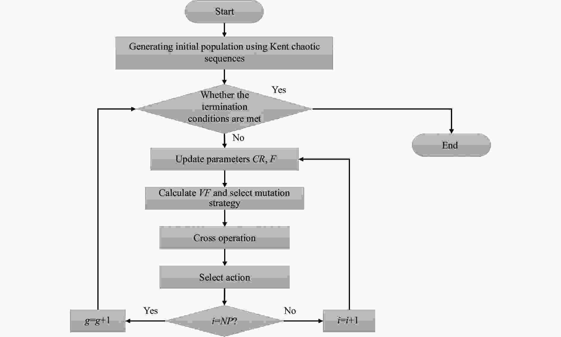
图 2 DSADE算法流程图
Figure 2. DSADE algorithm flowchart
步骤1:生成NP个Kent混沌序列,使用混沌序列产生初始种群X和Y;
步骤2:计算种群所有个体的适应度值和变异因子VF,初始化F和CR;
步骤3:针对不同个体根据变异因子VF选择对应的变异策略;
步骤4:执行交叉和选择操作;
步骤5:根据进化结果更新缩放比例因子F和交叉概率CR。
-
为了对比Kent混沌序列以及传统均匀分布随机生成的初始种群中个体基因在解空间中的均匀度,通过引入方差D来衡量初始数据的离散程度:
$$ \begin{array}{c}D=\dfrac{1}{n}\displaystyle\sum _{i=1}^{n}{\left({x}_{i}-\overline{x}\right)}^{2}\end{array} $$ (13) 假设初始种群中个体数NP为1000,个体中基因的取值上下界分别为10和0,个体基因维度n取0~100范围内间隔为20的5个样本采样点,分别使用Kent混沌序列和传统均匀分布生成初始种群,用种群个体方差均值$ \overline{D} $来衡量初始种群的均匀度:
$$ \begin{array}{c}\overline{D}=\dfrac{1}{NP}\displaystyle\sum _{i=1}^{NP}{D}_{i}\end{array} $$ (14) 式中:$ {D}_{i} $表示第i个个体的方差。
实验结果如表1所示,较好结果加粗表示,根据实验结果可知种群中个体取不同维度时Kent初始化方法生成的初始种群均匀度均优于随机生成的初始种群,说明Kent初始化方法相较于传统随机初始化方法能够生成更加均匀的初始种群。
表 1 初始化方法均匀度对比
Table 1. Uniformity comparison of initialization methods
n/dim 20 40 60 80 100 Kent 8.21 8.26 8.25 8.34 8.30 Random 7.53 7.84 8.03 8.09 8.16 -
为了验证文中提出的DSADE算法性能,选取常用的8种测试函数对算法性能进行了测试,测试函数介绍见表2。测试函数图像如图3所示,从图中可以看出,f1、f2、f3和f8为碗型函数,f5为谷型函数,f4、f6和f7为多峰函数。
表 2 标准测试函数
Table 2. Standard test function
Function Function expression Range Optimum $ {f}_{1} $ $ {\displaystyle\sum }_{i=1}^{n}{x}_{i}^{2} $ (−5.12,5.12) 0 $ {f}_{2} $ ${\displaystyle\sum }_{i=1}^{n}\left|{x}_{i}\right|+{\displaystyle\prod }_{i=1}^{n}\left|{x}_{i}\right|$ (−10,10) 0 $ {f}_{3} $ $ {\displaystyle\sum }_{i=1}^{n}{\left({\displaystyle\sum }_{j=1}^{i}{x}_{j}\right)}^{2} $ (−100,100) 0 $ {f}_{4} $ $ {\displaystyle\sum }_{i=1}^{n}[{x}_{i}^{2}-10\mathrm{cos}\left(2\pi {x}_{i}\right)+10] $ (−5.12,5.12) 0 $ {f}_{5} $ ${\displaystyle\sum }_{i=1}^{n-1}\left[{100\left({x}_{i}^{2}-{x}_{i+1}\right)}^{2}+{({x}_{i}-1)}^{2}\right]$ (−30,30) 0 $ {f}_{6} $ $ {\displaystyle\sum }_{i=1}^{n}|{x}_{i}\mathrm{sin}\left({x}_{i}\right)+0.1{x}_{i}| $ (−10,10) 0 $ {f}_{7} $ ${\displaystyle\sum }_{i=1}^{n}\frac{ {x}_{i}^{2} }{4\;000}-{\displaystyle\prod }_{i=1}^{n}\mathrm{cos}\left(\dfrac{ {x}_{i} }{\sqrt{i} }\right)+1$ (−5.12,5.12) 0 $ {f}_{8} $ $ {\displaystyle\sum }_{i=1}^{n}{x}_{i}^{10} $ (−5.12,5.12) 0 
图 3 测试函数图
Figure 3. Test function image
仿真实验结果基于Python3版本,计算机配置:16G内存和Inter Core i7处理器。对于所有的标准测试函数,算法的参数设置为:空间维数D=30,种群规模NP=100,缩放比例因子F=0.5,交叉概率CR=0.3,最大迭代次数1 000次。将8个测试函数作为适应度函数,分别使用DE/rand/1、DE/best/1、DE/current-to-best/1和DSADE 4种算法进行测试,每个测试函数独立优化50次,通过均值和方差衡量每种算法在标准函数求极值的收敛能力, 为保证优化算法的公平性,4种算法均采用Kent混沌初始化方法生成初始种群
表3为4种算法优化结果的均值和方差,较好结果加粗表示。从表3能够看出,文中提出的DSADE算法在所有测试函数中均表现较好,尤其在f4、f6这两个多峰函数的求解上,DSADE算法均取得了较好的结果,且最优结果在收敛精度方面均有数量级的提升,f7函数性能和DE/best/2最终优化结果相当,但实验中DSADE具有更快的收敛速度。综上,验证了DSADE算法在优化复杂非线性问题上的有效性。
表 3 标准测试函数实验结果
Table 3. Experimental results of standard test function
Function DE/rand/2 DE/best/2 DE/current-to-best/1 DSADE Mean Std Mean Std Mean Std Mean Std $ {f}_{1} $ 2.59e-06 7.77e-06 1.58e-15 4.74e-15 3.95e-02 1.18e-03 9.96e-35 4.40e-35 $ {f}_{2} $ 4.60e-03 1.38e-03 1.15e-05 3.46e-05 1.99e+01 5.27e+01 2.88e-20 1.35e-20 $ {f}_{3} $ 4.73e+04 3.86e+04 1.80e+04 4.80e+04 7.26e+04 3.75e+04 2.00e-00 1.80e-00 $ {f}_{4} $ 3.31e+02 18.3e+03 7.87e+02 8.41e+02 1.03e+02 2.00e+01 2.16e+00 1.96e+00 $ {f}_{5} $ 2.34e+02 1.68e+02 2.40e+00 0.84e+01 3.72e+03 5.62e+03 1.89e+00 2.20e+00 $ {f}_{6} $ 8.85e+01 3.38e+01 9.46e-02 1.89e-02 9.49e+01 2.38e+01 1.97e-18 1.37e-18 $ {f}_{7} $ 6.38e-04 1.28e-04 0.00e+00 0.00e+00 3.69e-01 6.30e-01 0.00e+00 0.00e+00 $ {f}_{8} $ 1.13e-13 2.26e-13 4.82e-43 9.64e-43 9.91e-02 1.94e-02 4.32e-75 7.24e-74 -
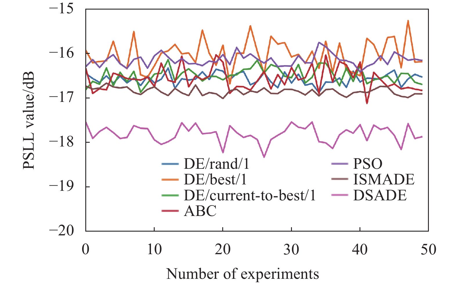
为验证文中提出的DSADE算法在太赫兹MIMO阵列优化方面的性能,设计了阵列优化仿真对比实验,在对比实验中采用变异策略分别为DE/rand/1、DE/best/1和DE/current-to-best/1的标准DE算法、人工蜂群算法ABC、粒子群算法PSO、ISMADE[26]以及文中提出的DSADE分别对阵列进行优化,相关优化算法参数设置如表4所示。
表 4 优化算法参数设置
Table 4. Optimization algorithm parameter setting
Algorithm Related parameters F CR DE/rand/1 0.5 0.9 DE/best/1 0.5 0.9 DE/current-to-best/1 0.5 0.9 ISMADE Self-adaption 0.9 DSADE Self-adaption Self-adaption ABC Leading bee Following bee 50%NP 50%NP PSO C1 C2 w 2 2 0.8 仿真条件参数设置如下:太赫兹MIMO阵列发射单元频率为100 GHz,波长$ \lambda =3 \;{\rm{mm}} $,发射和接收均阵元分布在一维直线上且最小间距$ {d}_{\min} $为1个波长,发射阵元数为8个,$ {N}_{t}=8 $,接收阵元数为8个,$ {N}_{r}=8 $。种群规模NP=100,Z最大迭代次数G=1 000次,变异后个体越界采用镜像初始化,计算机相关配置同3.2节。实验中,除文中提出的改进差分进化算法DSADE使用Kent混沌初始化方法外,其余优化算法均使用随机初始化方法,对于太赫兹MIMO阵列的优化,每种算法独立运行50次,表5为不同算法优化结果的平均峰值旁瓣比PSLL的均值、方差以及最好优化结果,较好结果加粗表示,图4展示了DSADE算法优化前后太赫兹MIMO雷达阵列综合方向图,从图中能够明显看出旁瓣电平的抑制效果。表6为优化后的太赫兹MIMO阵列收发阵元位置。
表 5 仿真优化结果对比
Table 5. Comparison of simulation optimization results
Algorithm Ave/dB Std/$ {\mathrm{d}\mathrm{B}}^{2} $ Best/dB DE/rand/1 −16.57 1.24e-1 −16.88 DE/best/1 −16.03 3.21e-1 −16.68 DE/current-to-best/1 −16.49 1.70e-1 −16.87 ABC −16.55 2.49e-1 −17.12 PSO −16.15 1.33e-1 −16.41 ISMADE −16.87 0.80e-1 −17.01 DSADE −17.81 1.82e-1 −18.33 
图 4 (a) MIMO阵列综合方向图(优化前);(b) MIMO阵列综合方向图(DSADE算法优化后)
Figure 4. (a) MIMO array comprehensive directional map (before optimization); (b) MIMO array comprehensive directional pattern (optimized by DSADE algorithm)
表 6 优化后MIMO阵列位置(单位:cm)
Table 6. Optimized MIMO array position(Unit: cm)
$ {x}_{1} $ $ {x}_{2} $ $ {x}_{3} $ $ {x}_{4} $ $ {x}_{5} $ $ {x}_{6} $ $ {x}_{7} $ $ {x}_{8} $ 0 0.8706 1.5816 2.4426 3.6719 5.0402 6.4105 6.9 $ {y}_{1} $ $ {y}_{2} $ $ {y}_{3} $ $ {y}_{4} $ $ {y}_{5} $ $ {y}_{6} $ $ {y}_{7} $ $ {y}_{8} $ 0.3 1.1895 2.7518 3.0651 4.7337 5.7784 6.0973 7.2 从表5的太赫兹MIMO阵列优化结果可以看出,文中提出的双变异自适应差分进化算法DSADE在旁瓣电平优化中具有更高的优化精度,优化效果最好。图5展示了不同算法单次优化的收敛结果,从图中能够看出,文中提出的DSADE算法在第150次迭代左右就能收敛到其他算法的最优结果,说明DSADE算法不仅收敛性能明显优于其他算法,同时收敛速度也更快。图6为50次优化实验结果对比图,从图中能够看出文中提出的算法性能明显优于其他算法。
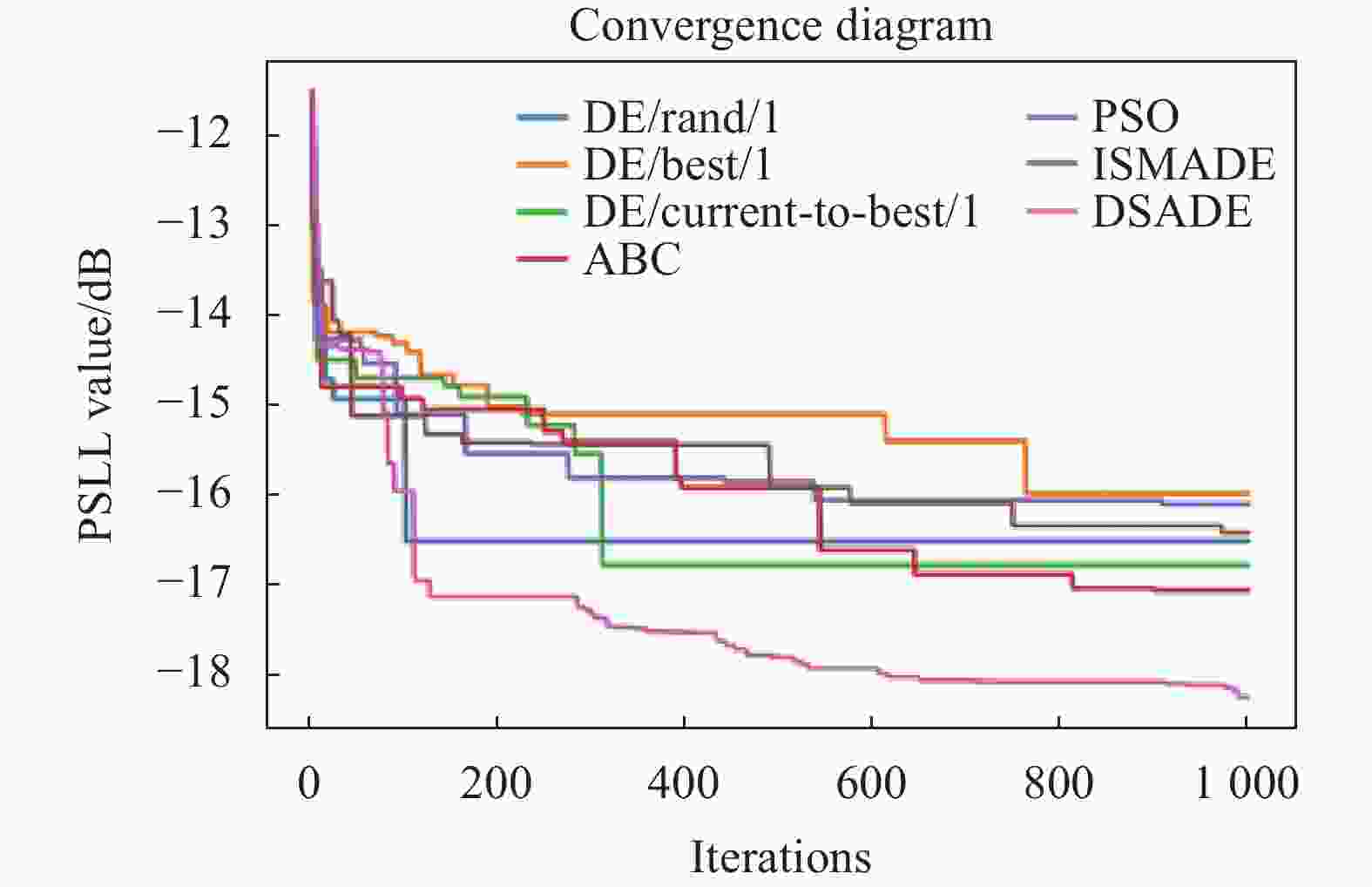
图 5 优化算法收敛对比图
Figure 5. Optimization algorithm convergence comparison chart

图 6 实验结果对比图
Figure 6. Comparison chart of experimental results
-
文中提出了一种改进的双变异自适应差分进化算法,用于优化太赫兹波段MIMO雷达阵列,通过改变发射和接收阵元在阵列实孔径中位置达到抑制旁瓣电平、将辐射能量集中到主瓣的作用。算法改进方面:首先引入了Kent混沌初始化方法使阵列初始位置在解空间中更加均匀分布;其次,在变异阶段提出了自适应变异因子VF,用来控制算法根据迭代周期以及个体适应度值来选择不同的变异策略,平衡了算法的全局探索和局部开采的能力;此外,针对差分进化算法中的参数缩放比例因子F和交叉概率CR提出了一种参数自适应调节方式,使参数能够根据个体进化情况自适应地进行调节。实验部分,首先对比验证了Kent混沌序列初始化方法初始的种群相较于随机初始化方法在解空间中更加均匀;然后通过8组测试函数的对比实验验证了DSADE算法的优化收敛能力;最后设计了太赫兹波段MIMO阵列仿真对比实验,通过7种智能优化算法的对比实验验证了文中提出的DSADE算法针对太赫兹MIMO雷达阵列优化具有更高的优化精度。此外,通过分析可知当阵元间距与波长同比例放大时,优化算法也同样适用,因此,该算法也能够扩展到其他波段的MIMO阵列雷达优化设计。
Optimization of terahertz MIMO array radar based on dual strategy differential evolution algorithm
-
摘要: 太赫兹波由于其高分辨率、高穿透性和高安全性等特点,太赫兹MIMO阵列雷达结合了多输入多输出(Multiple-Input Multiple-Output,MIMO)阵列技术,能够实现实时高分辨率成像,在人体安检等领域得到了广泛应用。然而,由于太赫兹波波长更短以及稀疏布阵使阵元间距远大于发射信号半波长,使阵列雷达波束方向图中出现高栅旁瓣电平问题,影响成像质量。针对该问题,文中在差分进化算法的基础上提出了一种双策略自适应差分进化算法(Dual Strategy Adaptive Differential Evolution,DSADE)用于阵列优化:首先,改进种群初始化方法,使用Kent混沌序列生成初始种群,该方法能够使初始个体基因在解空间中分布更加均匀;其次,提出了一种双变异策略,使算法能够根据迭代次数和个体适应度值选择合适的变异策略;最后,对参数进行了自适应改进,使参数能够根据个体进化情况进行自主调整。为验证DSADE算法收敛性选取了8组标准函数对算法进行了测试,DSADE算法在所有测试函数上均能取得最好的收敛效果。此外,使用DSADE算法对太赫兹MIMO雷达进行了仿真优化实验,该算法比优化效果最好的人工蜂群算法的归一化峰值旁瓣电平比值降低了1.21 dB。实验结果表明:文中提出的DSADE算法能够有效抑制太赫兹MIMO阵列雷达的峰值旁瓣电平,优化后的阵列雷达具有更低的旁瓣电平水平。Abstract:
Objective In recent years, terahertz radar has been widely used in the fields such as human security and non-destructive testing due to its advantages of high resolution, high penetration, and high safety. Researchers have proposed terahertz MIMO array radar from the perspective of improving imaging speed. This radar combines the spatial division multiplexing technology of MIMO arrays to achieve fast and real-time imaging. However, due to the short wavelength of terahertz waves and the sparse design of MIMO arrays, the array element spacing is too large, resulting in high gate sidelobe levels in the radar beam pattern, which affects imaging quality. Optimizing the array position through optimization algorithms can effectively solve this problem, but previous research is mainly focused on optimizing low-frequency MIMO array radars, while high-frequency terahertz MIMO array radars may encounter more severe high gate sidelobe level problems. Therefore, it is necessary to design optimization algorithms with higher optimization accuracy for this band. Therefore, from the perspective of solving this problem, this paper first abstracts the optimization model of terahertz MIMO linear array, and then proposes a dual strategy adaptive differential evolution for array optimization based on the optimization characteristics of the model. Methods A multi-constraint optimization model is established with the goal of reducing the peak sidelobe level ratio based on the optimization characteristics of terahertz MIMO arrays. Using Kent chaotic sequences to generate an initial population, this method can make the distribution of initial individual genes more uniform in the solution space. A dual mutation strategy was proposed to enable the algorithm to select appropriate mutation strategies based on the number of iterations and individual fitness values. Adaptive improvements have been made to the parameters, allowing them to be autonomously adjusted based on individual evolution. The convergence performance of the algorithm was tested through standard functions, and the effectiveness of the algorithm for terahertz MIMO array optimization was tested through simulation experiments. Results and Discussions The DSADE algorithm proposed in this paper has the best optimization effect on the 8 transmitting and 8 receiving terahertz MIMO array antenna, and the optimized minimum peak sidelobe level ratio is 1.32 dB lower than the ISMADE algorithm (Tab.5). It can be clearly seen from Fig.4 that the DSADE algorithm effectively suppresses the gate sidelobe level in the directional synthesis map of the MIMO array. The comparison of the 50 optimization results (Fig.6) also shows that the optimization performance of the DSADE algorithm is significantly better than other algorithms. It has been proven that this algorithm can effectively optimize terahertz MIMO arrays, suppress gate sidelobe levels, and improve imaging quality. Conclusions A portable infrared target simulation system is designed with working wavelengths of 3-5 μm and 8-14 μm. This system has the characteristics of simple structure, adjustable wavelength, rich targets, and clear and stable imaging. The wavefront quality of the system was analyzed using Zemax software, and at 4 μ the PV value of the center field of view in the m-band is 0.0132λ. The root mean square value is 0.0038λ, at 12 μ the photovoltaic value of the center field of view in the m-band is 0.0044λ. The mean square difference is 0.0013λ. An optical mechanical thermal analysis was conducted on the collimation system, and at a temperature difference of 30 ℃, the deformation caused by the mechanical structure was much greater than that of the primary and secondary mirrors themselves, reaching 10% μ. In the order of m, the imaging results have significant defocusing errors, which can be compensated for by temperature changes through refocusing the target disk in an adjustable three-dimensional position. The imaging function of the system was tested. For targets of different shapes, the system can generate clear and recognizable images, providing stable simulated targets for infrared detection equipment. -
Key words:
- differential evolution /
- MIMO /
- terahertz radar /
- peak sidelobe level
-
图 4 (a) MIMO阵列综合方向图(优化前);(b) MIMO阵列综合方向图(DSADE算法优化后)
Figure 4. (a) MIMO array comprehensive directional map (before optimization); (b) MIMO array comprehensive directional pattern (optimized by DSADE algorithm)
表 1 初始化方法均匀度对比
Table 1. Uniformity comparison of initialization methods
n/dim 20 40 60 80 100 Kent 8.21 8.26 8.25 8.34 8.30 Random 7.53 7.84 8.03 8.09 8.16  下载: 导出CSV
表 2 标准测试函数
Table 2. Standard test function
Function Function expression Range Optimum $ {f}_{1} $ $ {\displaystyle\sum }_{i=1}^{n}{x}_{i}^{2} $ (−5.12,5.12) 0 $ {f}_{2} $ ${\displaystyle\sum }_{i=1}^{n}\left|{x}_{i}\right|+{\displaystyle\prod }_{i=1}^{n}\left|{x}_{i}\right|$ (−10,10) 0 $ {f}_{3} $ $ {\displaystyle\sum }_{i=1}^{n}{\left({\displaystyle\sum }_{j=1}^{i}{x}_{j}\right)}^{2} $ (−100,100) 0 $ {f}_{4} $ $ {\displaystyle\sum }_{i=1}^{n}[{x}_{i}^{2}-10\mathrm{cos}\left(2\pi {x}_{i}\right)+10] $ (−5.12,5.12) 0 $ {f}_{5} $ ${\displaystyle\sum }_{i=1}^{n-1}\left[{100\left({x}_{i}^{2}-{x}_{i+1}\right)}^{2}+{({x}_{i}-1)}^{2}\right]$ (−30,30) 0 $ {f}_{6} $ $ {\displaystyle\sum }_{i=1}^{n}|{x}_{i}\mathrm{sin}\left({x}_{i}\right)+0.1{x}_{i}| $ (−10,10) 0 $ {f}_{7} $ ${\displaystyle\sum }_{i=1}^{n}\frac{ {x}_{i}^{2} }{4\;000}-{\displaystyle\prod }_{i=1}^{n}\mathrm{cos}\left(\dfrac{ {x}_{i} }{\sqrt{i} }\right)+1$ (−5.12,5.12) 0 $ {f}_{8} $ $ {\displaystyle\sum }_{i=1}^{n}{x}_{i}^{10} $ (−5.12,5.12) 0
下载: 导出CSV
表 3 标准测试函数实验结果
Table 3. Experimental results of standard test function
Function DE/rand/2 DE/best/2 DE/current-to-best/1 DSADE Mean Std Mean Std Mean Std Mean Std $ {f}_{1} $ 2.59e-06 7.77e-06 1.58e-15 4.74e-15 3.95e-02 1.18e-03 9.96e-35 4.40e-35 $ {f}_{2} $ 4.60e-03 1.38e-03 1.15e-05 3.46e-05 1.99e+01 5.27e+01 2.88e-20 1.35e-20 $ {f}_{3} $ 4.73e+04 3.86e+04 1.80e+04 4.80e+04 7.26e+04 3.75e+04 2.00e-00 1.80e-00 $ {f}_{4} $ 3.31e+02 18.3e+03 7.87e+02 8.41e+02 1.03e+02 2.00e+01 2.16e+00 1.96e+00 $ {f}_{5} $ 2.34e+02 1.68e+02 2.40e+00 0.84e+01 3.72e+03 5.62e+03 1.89e+00 2.20e+00 $ {f}_{6} $ 8.85e+01 3.38e+01 9.46e-02 1.89e-02 9.49e+01 2.38e+01 1.97e-18 1.37e-18 $ {f}_{7} $ 6.38e-04 1.28e-04 0.00e+00 0.00e+00 3.69e-01 6.30e-01 0.00e+00 0.00e+00 $ {f}_{8} $ 1.13e-13 2.26e-13 4.82e-43 9.64e-43 9.91e-02 1.94e-02 4.32e-75 7.24e-74
下载: 导出CSV
表 4 优化算法参数设置
Table 4. Optimization algorithm parameter setting
Algorithm Related parameters F CR DE/rand/1 0.5 0.9 DE/best/1 0.5 0.9 DE/current-to-best/1 0.5 0.9 ISMADE Self-adaption 0.9 DSADE Self-adaption Self-adaption ABC Leading bee Following bee 50%NP 50%NP PSO C1 C2 w 2 2 0.8
下载: 导出CSV
表 5 仿真优化结果对比
Table 5. Comparison of simulation optimization results
Algorithm Ave/dB Std/$ {\mathrm{d}\mathrm{B}}^{2} $ Best/dB DE/rand/1 −16.57 1.24e-1 −16.88 DE/best/1 −16.03 3.21e-1 −16.68 DE/current-to-best/1 −16.49 1.70e-1 −16.87 ABC −16.55 2.49e-1 −17.12 PSO −16.15 1.33e-1 −16.41 ISMADE −16.87 0.80e-1 −17.01 DSADE −17.81 1.82e-1 −18.33
下载: 导出CSV
表 6 优化后MIMO阵列位置(单位:cm)
Table 6. Optimized MIMO array position(Unit: cm)
$ {x}_{1} $ $ {x}_{2} $ $ {x}_{3} $ $ {x}_{4} $ $ {x}_{5} $ $ {x}_{6} $ $ {x}_{7} $ $ {x}_{8} $ 0 0.8706 1.5816 2.4426 3.6719 5.0402 6.4105 6.9 $ {y}_{1} $ $ {y}_{2} $ $ {y}_{3} $ $ {y}_{4} $ $ {y}_{5} $ $ {y}_{6} $ $ {y}_{7} $ $ {y}_{8} $ 0.3 1.1895 2.7518 3.0651 4.7337 5.7784 6.0973 7.2
下载: 导出CSV
-
[1] Sheen D, Mcmakin D, Hall T. Near-field three-dimensional radar imaging techniques and applications [J]. Applied Optics, 2010, 49(19): 83-93. doi: 10.1364/AO.49.000E83 [2] Charvat G L, Kempel L C, Rothwell E J, et al. A through-dielectric ultrawideband (UWB) switched-antenna-array radar imaging system [J]. IEEE Transactions on Antennas and Propagation, 2012, 60(11): 5495-5500. doi: 10.1109/TAP.2012.2207663 [3] Fishler E, Haimovich A, Blum R, et al. Performance of MIMO radar systems: Advantages of angular diversity[C]//Conference Record of the Thirty-Eighth Asilomar Conference on Signals, Systems and Computers, 2004. IEEE, 2004, 1: 305-309. [4] Li J, Stoica P. MIMO radar with colocated antennas [J]. IEEE Signal Processing Magazine, 2007, 24(5): 106-114. doi: 10.1109/MSP.2007.904812 [5] Bliss D W, Forsythe K W. Multiple-input multiple-output (MIMO) radar and imaging: degrees of freedom and resolution[C]//The Thrity-Seventh Asilomar Conference on Signals, Systems & Computers, 2003. IEEE, 2003, 1: 54-59. [6] Fuhrmann D R, San Antonio G. Transmit beamforming for MIMO radar systems using signal cross-correlation [J]. IEEE Transactions on Aerospace and Electronic Systems, 2008, 44(1): 171-186. doi: 10.1109/TAES.2008.4516997 [7] Forsythe K W, Bliss D W, Fawcett G S. Multiple-input multiple-output (MIMO) radar: Performance issues[C]//Conference Record of the Thirty-Eighth Asilomar Conference on Signals, Systems and Computers, IEEE, 2004, 1: 310-315. [8] Cheng B, Cui Z, Lu B, et al. 340-GHz 3-D imaging radar with 4 Tx-16 Rx MIMO array [J]. IEEE Transactions on Terahertz Science and Technology, 2018, 8(5): 509-519. doi: 10.1109/TTHZ.2018.2853551 [9] Oliveri G, Massa A. Genetic algorithm (GA)-enhanced almost difference set (ADS)-based approach for array thinning [J]. IET Microwaves, Antennas & Propagation, 2011, 5(3): 305-315. [10] Chen K, Chen H, Wang L, et al. Modified real GA for the synthesis of sparse planar circular arrays [J]. IEEE Antennas and Wireless Propagation Letters, 2016, 15: 274-277. doi: 10.1109/LAWP.2015.2440432 [11] Dai D, Yao M, Ma H, et al. An effective approach for the synthesis of uniformly excited large linear sparse array [J]. IEEE Antennas and Wireless Propagation Letters, 2018, 17(3): 377-380. doi: 10.1109/LAWP.2018.2790907 [12] Bhattacharya R, Bhattacharyya T K, Garg R. Position mutated hierarchical particle swarm optimization and its application in synthesis of unequally spaced antenna arrays [J]. IEEE Transactions on Antennas and Propagation, 2012, 60(7): 3174-3181. doi: 10.1109/TAP.2012.2196917 [13] Bai Y Y, Xiao S, Liu C, et al. A hybrid IWO/PSO algorithm for pattern synthesis of conformal phased arrays [J]. IEEE Transactions on Antennas and Propagation, 2012, 61(4): 2328-2332. [14] Sun G, Liu Y, Chen Z, et al. Radiation beam pattern synthesis of concentric circular antenna arrays using hybrid approach based on cuckoo search [J]. IEEE Transactions on Antennas and Propagation, 2018, 66(9): 4563-4576. doi: 10.1109/TAP.2018.2846771 [15] Price K V, Storn R M, Lampinen J A. The differential evolution algorithm [J]. Differential Evolution: A Practical Approach to Global Optimization, 2005: 37-134. [16] Guan B, Zhao Y, Li Y. DESeeker: detecting epistatic interactions using a two-stage differential evolution algorithm [J]. IEEE Access, 2019, 7: 69604-69613. doi: 10.1109/ACCESS.2019.2917132 [17] Zhao Y, Wang G. A dynamic differential evolution algorithm for the dynamic single-machine scheduling problem with sequence-dependent setup times [J]. Journal of the Operational Research Society, 2020, 71(2): 225-236. doi: 10.1080/01605682.2019.1596591 [18] Son N N, Van Kien C, Anh H P H. Parameters identification of Bouc-Wen hysteresis model for piezoelectric actuators using hybrid adaptive differential evolution and Jaya algorithm [J]. Engineering Applications of Artificial Intelligence, 2020, 87: 103317. doi: 10.1016/j.engappai.2019.103317 [19] Slowik A, Bialko M. Training of artificial neural networks using differential evolution algorithm[C]//Conference on Human System Interactions, IEEE, 2008: 60-65. [20] Adeyemo J, Otieno F. Differential evolution algorithm for solving multi-objective crop planning model [J]. Agricultural Water Management, 2010, 97(6): 848-856. doi: 10.1016/j.agwat.2010.01.013 [21] Khodier M M, Christodoulou C G. Linear array geometry synthesis with minimum sidelobe level and null control using particle swarm optimization [J]. IEEE Transactions on Antennas and Propagation, 2005, 53(8): 2674-2679. doi: 10.1109/TAP.2005.851762 [22] 陈刚. 稀布阵列 MIMO 雷达成像技术研究[D]. 南京: 南京理工大学, 2014. Chen Gang. Research on Techniques for Sparse ArrayMIMO Radar Imaging[D]. Nanjing: Nanjing University of Science & Technology, 2014. (in Chinese) [23] Chen K, Yun X, He Z, et al. Synthesis of sparse planar arrays using modified real genetic algorithm [J]. IEEE Transactions on Antennas and Propagation, 2007, 55(4): 1067-1073. doi: 10.1109/TAP.2007.893375 [24] Liu H, Zhao H, Li W, et al. Synthesis of sparse planar arrays using matrix mapping and differential evolution [J]. IEEE Antennas and Wireless Propagation Letters, 2016, 15: 1905-1908. doi: 10.1109/LAWP.2016.2542882 [25] Dai D, Yao M, Ma H, et al. An asymmetric mapping method for the synthesis of sparse planar arrays [J]. IEEE Antennas and Wireless Propagation Letters, 2017, 17(1): 70-73. [26] Fan S, Xie X, Zhou X. Optimum manipulator path generation based on improved differential evolution constrained optimization algorithm [J]. Int J Adv Robot Syst, 2019, 16(5): 1-9. -

 点击查看大图

计量
- 文章访问数: 133
- HTML全文浏览量: 31
- PDF下载量: 28
- 被引次数: 0

