


 下载:
下载:


-
由于水下激光通信具有高速率、保密性强等优点,众多研究学者对光束在海洋湍流中的传输特性展开了大量研究[1-4]。此外,由于涡旋光不同拓扑荷数的轨道角动量(Orbital Angular Momentum, OAM)可以进行复用[5],这将会大大增加系统容量。涡旋光束在水下传输时会受到海洋湍流的影响,因此研究涡旋光束在海洋湍流中的传输具有十分重要的意义。
利用相位屏模拟随机介质引起的波前畸变是最常用的数值仿真方法。最常见的三种产生湍流相位屏的方法分别是功率谱反演法[6]、Zernike多项式法[7]和分形法[8]。早在1976年,Fleck就利用多相位屏法模拟湍流[9]。由于功率谱反演法低频信息不足的缺点,Lane等人[10]提出了次谐波补偿法。利用相位屏法模拟光束在海洋湍流中传输的研究逐渐展开。Farwell等人[11]利用海洋湍流功率谱模型及多相位屏法模拟了高斯光束在海洋湍流中的传输,并分析了闪烁特性。杨天星等人[12]利用Nikishov提出的海洋湍流功率谱模型构建了水平路径上海洋湍流随机相位屏,并利用相位结构函数和探测概率验证了相位屏的准确性。牛超君等人[13]利用功率谱反演法建立海洋湍流随机相位屏,并分别计算了单光束和阵列光束的光束漂移和闪烁指数。Pan等人[14]分别采用功率谱反演法和Zernike多项式法构建了海洋湍流随机相位屏并利用相位结构函数验证了相位屏的准确性。张凯宁等人[15]利用分步相位屏方法仿真分析了涡旋光束在海洋湍流中的闪烁因子。杨祎等人[3]基于复合海水信道湍流香味平模型仿真了湍流外尺度对高斯光束的影响。以上利用相位屏法对光束在海洋湍流中传输的研究是基于水平路径下开展的,相对缺少光束经斜程海洋湍流路径下的传输研究。
因此,文中在斜程海洋湍流功率谱的基础上采用功率谱反演法构建海洋湍流随机相位屏并用次谐波法对缺失的低频信息进行补偿。结合斜程海洋湍流功率谱的相位结构函数验证构建相位屏的准确性,利用相位屏搭建斜程海洋湍流上行传输链路模型,数值仿真并分析不同天顶角和海洋湍流参数对准直高斯涡旋光束光强及相位分布、光束漂移、轴上闪烁指数和长曝光光斑半径的影响。
-
功率谱反演法产生海洋湍流随机相位屏的方法如下:首先生成一个零均值、单位方差的复高斯随机数矩阵,然后用海洋湍流相位扰动的功率谱密度函数对其滤波,最后通过傅里叶逆变换得到海洋湍流随机相位屏。根据相位屏的相位频谱和海洋湍流功率谱之间的关系可以得到光束在垂直于传播方向(z轴方向)上任意切片海水相位频谱为[14]:
$$ {F_\phi }\left( {{\kappa _x},{\kappa _y}} \right) = 2\pi {k^2}\Delta z{\varPhi _n}\left( {\kappa ,h} \right) $$ (1) 式中:k = 2π /λ是光束的波数; Δz为第i个与第i + 1个斜程路径下海洋湍流随机相位屏的湍流层厚度或光束的传播距离,Φn(κ, h)为斜程海洋湍流功率谱模型,其表达式为[16]:
$$ \begin{split} {\varPhi _n}(\kappa ,h) =& \frac{{\left[ {1 + {C_1}{{\left( {\kappa \eta } \right)}^{2/3}}} \right]}}{{4\pi {{\left( {{\kappa ^2} + \kappa _0^2} \right)}^{11/6}}}}\left\{ {{C_T}^2(h)\exp \left[ { - \frac{{{{\left( {\kappa \eta } \right)}^2}}}{{R_T^2}}} \right]}+ \right. \\ & \left. { {C_S}^2(h)\exp \left[ { - \frac{{{{\left( {\kappa \eta } \right)}^2}}}{{R_S^2}}} \right] - {C_{TS}}^2(h)\exp \left[ { - \frac{{{{\left( {\kappa \eta } \right)}^2}}}{{R_{TS}^2}}} \right]} \right\} \\ \end{split} $$ (2) 式中:κ 是空间波数;η 是海洋湍流的Kolmogorov微尺度;κ0 = 1/L0;L0是海洋湍流的Kolmogorov外尺度;C1是4.6~5的无量纲参数[17];CT2(h) = A2βχT(h)ε−1/3(h),A = 2.6×10⁻⁴ liter/(°),β = 0.72是Obukhov–Corrsin常数;χT(h)是随深度变化的温度耗散率;ε (h)是随深度变化的单位质量流体的海洋湍流动能耗散率;h是海水深度,CS2(h) = B2βχS(h)ε −1/3(h)是斜程海洋湍流的盐度结构参数,在上层海洋中盐度几乎不随海水深度变化而变化[18],因此斜程路径中均方盐度耗散率χS(h)可以近似为水平路径中的均方盐度耗散率χS,则有χS(h)≈χS=A2χT/B2ω2,B = 1.75×10⁻⁴ liter/gram;CTS2(h) = 2ABβχTS(h) ε −1/3(h)是斜程海洋湍流的温盐结构参数,χTS(h)=[KT+KS][ χT(h)χS(h)/4KTKS]1/2是随深度变化的海洋湍流均方温盐耦合耗散率;Rj =31/2[Wj −1/3+1/(9Wj)]3/2/Q3/2 (j = T, S, TS) , Q是范围在2.3~3.6之间变化的无量纲常量,Wj ={[Prj2/(6βQ−2)2−Prj/(81βQ−2)]1/2−[1/27−Prj/(6Q−2β)]}1/3 (j = T, S, TS),PrT和PrS分别是温度和盐度的Pandtl常数[16],且PrTS = 2 PrTPrS/(PrT+PrS)。
斜程海洋湍流路径下随海水深度变化的均方温度耗散率和动能耗散率分别为[16]:
$$ {\chi _T}\left( h \right) = \left\{ {\begin{array}{*{20}{c}} {{{\left( {J_b^0} \right)}^2}{{\left( {{h^2} + 0.48} \right)}^{ - 1/2}}/\left( {c_\rho ^2\rho _w^2{u_w}} \right),W \leqslant 7\;{\rm{m/s}}} \\ {{{\left( {T_0'} \right)}^2}{u_w}^{3/2}{{\left( {{h^2} + 0.48} \right)}^{ - 1/4}}/\sqrt {v\alpha } ,W > 7\;{\rm{m/s}}} \end{array}} \right. $$ (3) $$ \varepsilon \left( h \right) = \left( {C\vartheta {u^3} + D{{\left( {W\sqrt {{C_D}{\rho _a}/{\rho _w}} } \right)}^3}/\alpha } \right)/h $$ (4) 式中:cρ 是比热;$J_b^0 $是表面热浮力通量;uw 是海水侧摩擦速度;$T_0^{\prime} $湍流温度波动源;ν 是动能粘度系数;C = 0.004是潮汐混合系数;D = 0.023是风混合系数;W是风速;ρa是空气密度;ρw是海水密度;ϑ 是与海水深度成正比的最大涡流尺度;α = 0.41是von Karman常数;u是平均水深流速;CD 是风和海水表面之间的拖拽系数。
斜程海洋湍流路径下温度盐度贡献比可表示为[16]:
$$ \omega \left( h \right) = \frac{\omega }{{{{\left( {{h^2} + 0.48} \right)}^{{1 \mathord{\left/ {\vphantom {1 {\left( {4J} \right)}}} \right. } {\left( {4J} \right)}}}}}} $$ (5) 式中:J = 1代表弱风条件;J = 2代表强风条件;ω 为水平路径下温度盐度贡献比。
用Fϕ(κx, κy)对高斯随机复矩阵h(κx, κy)进行滤波,再进行傅里叶逆变换得到相位屏空间分布为:
$$ \begin{split}& \varphi \left( {x,y} \right) = \\& {C_2}\sum\nolimits_{{\kappa _x}} {\sum\nolimits_{{\kappa _y}} {{h_1}\left( {{\kappa _x},{\kappa _y}} \right)} } \sqrt {{F_\phi }\left( {{\kappa _x},{\kappa _y}} \right)} \exp \left[ {i\left( {{\kappa _x}x + {\kappa _y}y} \right)} \right] \end{split} $$ (6) 式中:C2 = (ΔκxΔκy)1/2是相位屏方差的常数因子;h1是N×N的复随机矩阵,在离散化的空间域内;x = mΔx,y = nΔy,Δx Δy分别为x, y方向的取样间隔,为了方便,设Δx = Δy,m、n为整数;在波数域内,κx = m'Δκx,κy = n'Δκy,Δκx Δκy为空间频域的取样间隔,Δκx = 2π/(MxΔx),Δκy = 2π/(MyΔy),Mx My分别为相位屏的栅格数目,则相位屏的表达式可写为:
$$ \begin{split} & {\phi _{\text{H}}}\left( {m\Delta x,n\Delta y} \right) = \\ & {C_2}\sum\limits_{m'} {\sum\limits_{n'} {h\left( {m',n'} \right)\sqrt {{F_\phi }\left( {m',n'} \right)} \exp \left[ {2\pi i\left( {\frac{{m'm}}{{{M_x}}} + \frac{{n'n}}{{{M_y}}}} \right)} \right]} } \\ \end{split} $$ (7) 由于功率谱反演法具有低频信息不足的缺陷,文中在功率谱反演法的基础上对产生的相位屏采用次谐波法进行低频补偿,低频次谐波频谱[12,14,19]可以表示为:
$$ {F_{sub}}\left( {{\kappa _x},{\kappa _y}} \right) = {\left( {q/N} \right)^{ - 2p}}{F_\phi }\left( {{\kappa _{lx}},{\kappa _{ly}}} \right) $$ (8) 式中:p为谐波次数;q为补偿阶数;N为低频次谐波的重叠补偿阶数;(q/N)−2p为低频次谐波权重,κlx = (q/N)−2pκx,κly = (q/N)−2pκy分别为x和y方向上的低频空间频率分量。离散化之后,低频次谐波相位屏表达式为:
$$ \begin{split} {\phi _L}\left( {m\Delta x,n\Delta y} \right)&= {\left[ {{{\left( {\frac{{2\pi }}{M}} \right)}^2}\tfrac{1}{{\Delta x\Delta y}}} \right]^{\tfrac{1}{2}}}\sum\limits_{p = 1}^{{M_P}} {\sum\limits_{m' = - \tfrac{{q - 1}}{2}}^{\tfrac{{q - 1}}{2}} {\sum\limits_{n' = - \tfrac{{q - 1}}{2}}^{\tfrac{{q - 1}}{2}} {h\left( {m',n'} \right)}}}\\ & {{{\sqrt {{F_{sub}}\left( {m',n'} \right)} } } } \times \exp \left[ {{\text{i}}2\pi {{\left( {\frac{q}{N}} \right)}^{ - p}}\left( {\frac{{m'm}}{{{M_x}}} + \frac{{n'n}}{{{M_y}}}} \right)} \right] \end{split} $$ (9) 式中:Mp代表补偿的总阶数。将公式(7)和(9)合并构成最终的海洋湍流随机相位屏,从而补偿了相位屏的低频部分。最终的相位屏可以表示为ϕ = ϕH + ϕL。
-
光束在海洋湍流中传输的影响可以近似认为是纯相位扰动[12],因此光束在斜程海洋湍流路径下传输的影响可以采用一系列的相位屏模拟。图1为光束通过海洋湍流随机相位屏上行传输链路模型示意图。
如图1所示,h0为上行传输链路中接收机所处海水深度,H=h0+ zcosζ,Δh = Δz·cosζ,从而可以得到斜程海洋湍流传输链路中每个相位屏的深度。准直高斯涡旋光束在笛卡尔坐标系下初始源平面的场[20]可以表示为:
$$ {U_0}\left( {{\boldsymbol{s}},z} \right) = {\left[ {{s_x} + i{s_y}{sgn} \left( l \right)} \right]^{\left| l \right|}} \cdot \exp \left[ { - \frac{{s_x^2 + s_y^2}}{{w_0^2}}} \right] $$ (10) 式中:s = (sx, sy)是源平面处的坐标;l是拓扑荷数;sgn(·)是符号函数;w0是光束的束腰半径;准直高斯涡旋光束在自由空间中的传输函数[21]为:
$$ {U_{prop}}\left( {{\kappa _x},{\kappa _y}} \right) = \exp \left[ {i\Delta z\left( {\kappa _r^2 - \kappa _x^2 - \kappa _y^2} \right)} \right] $$ (11) 式中:κr2= κx2+κy2,κx、κy分别为x轴、y轴方向上的空间频率分量。光束通过第一个相位屏后的光场表达式为:
$$ \begin{gathered} {U_{1 + }}\left( {x,y} \right) = \\ FF{T^{ - 1}}\left[ {FFT\left( {{U_0}} \right) \cdot {U_{prop}}\left( {{\kappa _x},{\kappa _y}} \right)} \right] \cdot \exp \left[ {i{\phi _1}\left( {x,y} \right)} \right] \\ \end{gathered} $$ (12) 式中:ϕ1(x, y)表示斜程海洋湍流上行传输链路中的第一个相位屏,FFT −1和FFT分别表示傅里叶反变换和傅里叶变换。当光束通过第二个相位屏后光场表达式为:
$$ \begin{gathered} {U_{2 + }}\left( {x,y} \right) = \\ FF{T^{ - 1}}\left[ {FFT\left( {{U_{1 + }}} \right) \cdot {U_{prop}}\left( {{\kappa _x},{\kappa _y}} \right)} \right] \cdot \exp \left[ {i{\phi _2}\left( {x,y} \right)} \right] \\ \end{gathered} $$ (13) 式中:ϕ2(x,y)表示斜程海洋湍流上行传输链路中的第二个相位屏。值得注意的是,在斜程海洋湍流链路中相位屏的深度变化会影响相位屏模拟数值的大小,因此,不同深度处的相位屏并不相同。当通过第二个相位屏后,以上过程将被重复直到穿过最后一个相位屏为止,最终的结果即为出射光束的场强分布。

图 1 光束通过海洋湍流相位屏上行传输链路模型示意图
Figure 1. Schematic diagram of the beam through phase screen in uplink transmission channel model of ocean turbulence
-
海洋湍流的统计特性可以用结构函数描述[12],通过对海洋湍流功率谱的相位结构函数与生成相位屏的相位结构函数的数值进行比较分析,验证生成相位屏的准确性。斜程路径下海洋湍流随机相位屏的相位结构函数[14]定义为:
$$ D(r) = \left\langle {{{\left[ {\varphi (\rho + r) - \varphi (\rho )} \right]}^2}} \right\rangle $$ (14) 式中:φ(ρ+r)和φ(ρ)分别是点ρ + r和点 ρ 的相位值,<·>是系综平均。斜程路径下海洋湍流功率谱相位结构函数的理论表达式[22-23]为:
$$ D\left( r \right) = \left\{ {\begin{array}{*{20}{c}} {2{{\left( {r/{r_0}} \right)}^2}{\text{ }},r < < \eta } \\ {2{{\left( {r/{r_0}} \right)}^{5/3}},r > > \eta } \end{array}} \right. $$ (15) 式中:η是海洋湍流内尺度;r0是海洋湍流的空间相干长度[24-25],可以表示为:
$$ {r_0} = {\left[ {1.118\;3\pi {k^2}\sec \left( \zeta \right)\left( {{\mu _T} + {\mu _S} - {\mu _{TS}}} \right)} \right]^{ - 3/5}},{r_0} > > \eta $$ (16) 其中:
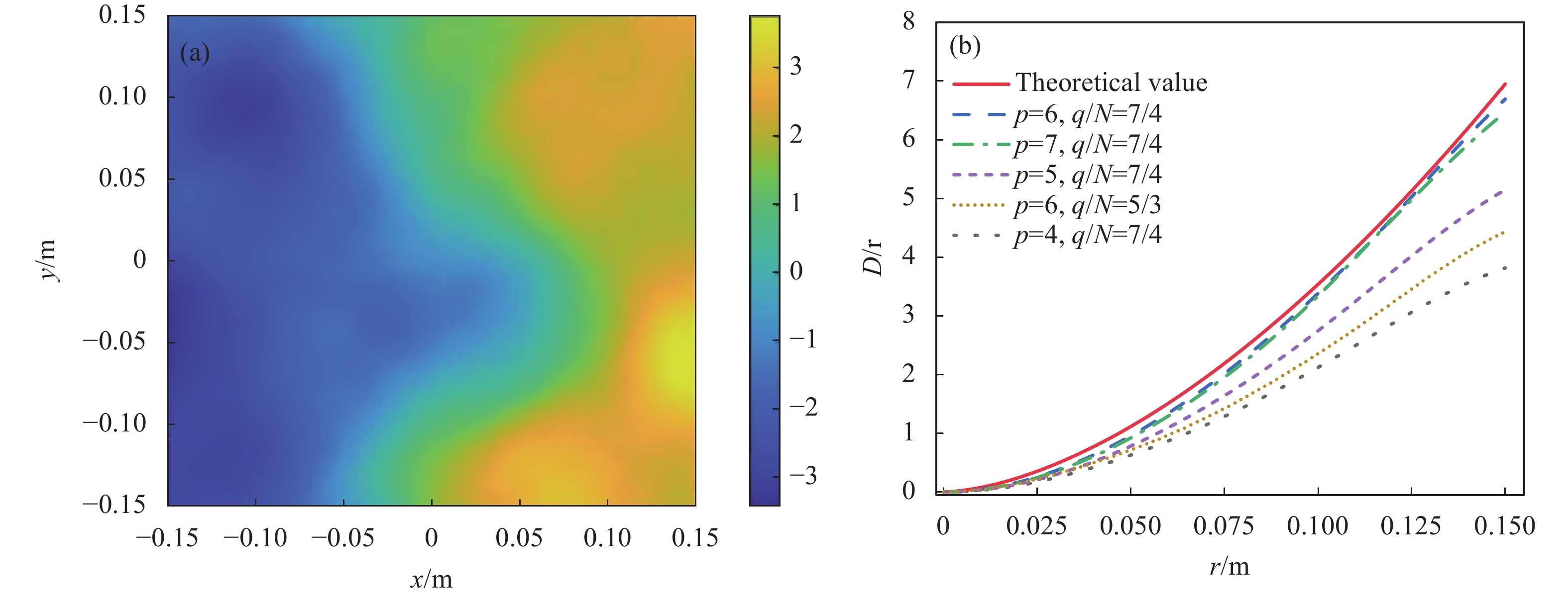
$$ {\mu _j} = \int\limits_{{h_0}}^H {C_j^2\left( h \right)} {\rm{d}}h,j = T,S,TS $$ (17) 斜程路径下海洋湍流相位屏仿真选取参数为:η = 0.001 m, uw = 0.0012 m/s,u = 0.5 m/s, T ′0 = 0.03 ℃,W = 1 m/s ,CD = 0.0015,ω = −3, ρa = 1.2 kg/m3,cρ = 3932 J·kg−1/℃, ρw = 1025 kg/m3, λ = 532 nm,L0 = 10 m,ϑ = 7×10⁻²,ζ = π/3 ,v = 0.0001 m2/s,Q = 2.35, J = 1, J0b = 6 W/m2 , w0 = 0.05 m, Δz = 20 m, l = 1, z = 20 m, 采样点数M = 1024, 相位屏尺寸L = 0.3 m。如无特殊说明仿真参数均为以上参数。将海洋湍流随机相位屏的中心点作为固定点,计算与相位屏中心点距离为0~r的点的相位均方差,然后取1000幅相位屏进行数学平均作为系综平均。以p = 6, q/N = 7/4的次谐波补偿法生成相位屏的二维图及对公式(14)和公式(15)进行数值仿真,得到斜程路径下海洋湍流随机相位屏相位结构仿真值与海洋湍流功率谱相位结构理论值的结果对比分别如图2(a)和图2(b)所示。从图2(a)可以看出,斜程路径下海洋湍流随机相位屏的相邻两点间的相位变化剧烈,即该相位屏具有丰富的高频成分,并且相位屏上的相位具有明显倾斜,因此该相位屏具有丰富的低频成分。从图2(b)中可以看出,当p = 6, q/N = 7/4时斜程路径下海洋湍流随机相位屏相位结构函数的仿真值与海洋湍流功率谱相位结构函数的理论值较为逼近,且在低频处也较为贴合,因此可以验证斜程路径下海洋湍流随机相位屏的准确性。
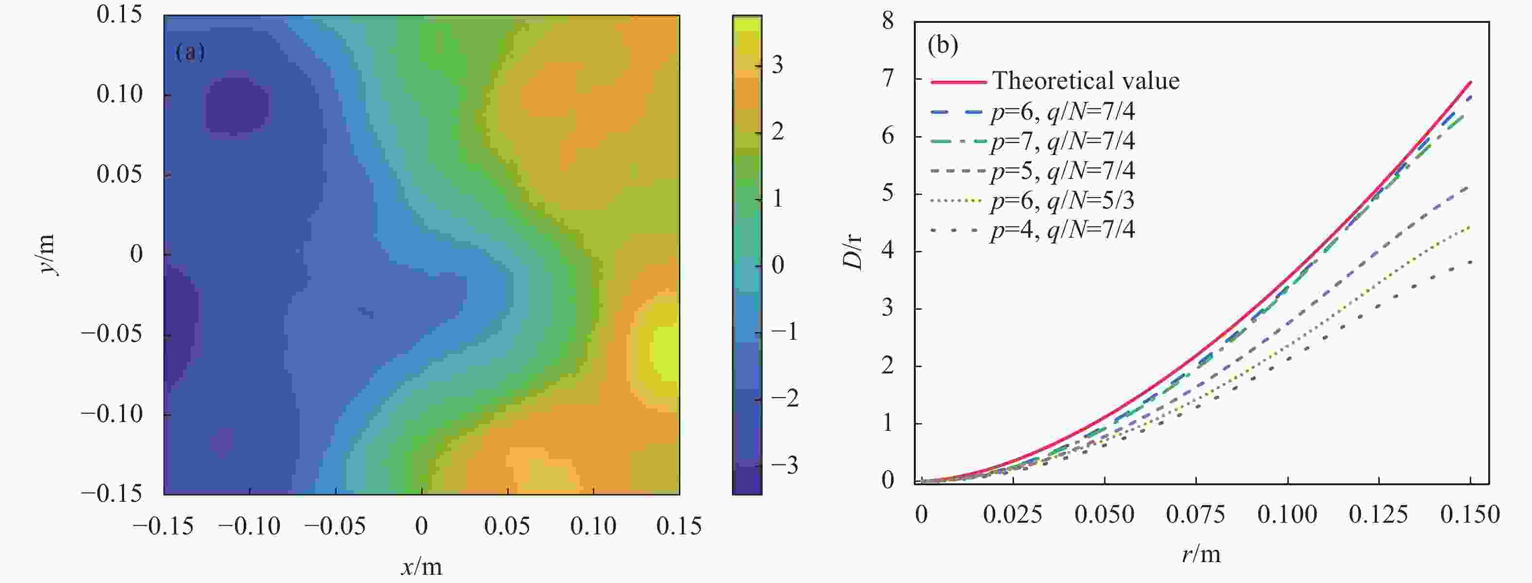
图 2 海洋湍流随机相位屏二维图及相位结构函数验证图。 (a)相位屏二维图; (b)相位结构函数验证图
Figure 2. Two-dimensional diagram of random ocean turbulence. (a) Phase screen; (b) Phase structure function curves
-
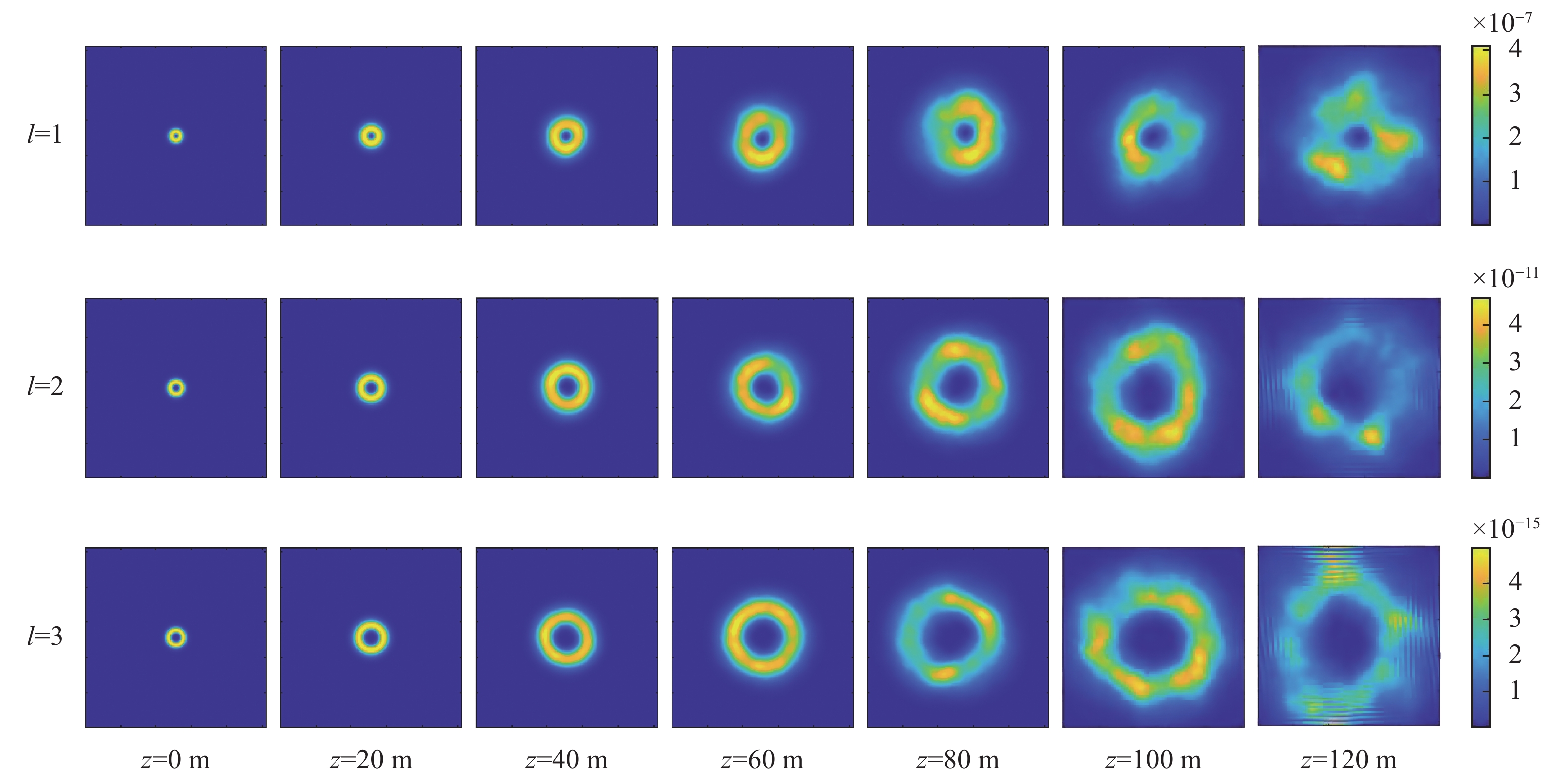
图3所示为弱风条件下准直高斯涡旋光束在不同拓扑荷数时光斑强度随传输距离变化的光斑分布图。从图3中可以看出,在斜程海洋湍流中随着传输距离的增大,光束的光斑逐渐开始破碎,表明随着传输距离增大光束受到海洋湍流的影响增大。造成这一现象的原因是当接收机的位置和天顶角的大小固定不变时,随着传输距离增大发射机所处的海水深度增加,盐度梯度变化要大于温度梯度变化且盐度变化主导的海洋湍流要强于温度变化主导的海洋湍流。此外,涡旋光束的光斑半径随着拓扑荷数及传输距离的增大而增大。

图 3 准直高斯涡旋光束在斜程海洋湍流中不同传输距离处的光斑强度分布情况
Figure 3. Intensity profiles of collimated Gaussian vortex beam at different propagation distance in ocean turbulence of slant path
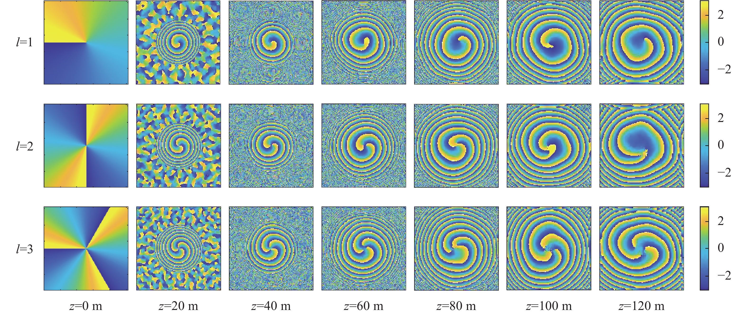
图4所示为弱风条件下准直高斯涡旋光束在不同拓扑荷数时相位随传输距离变化的相位分布图。从图4中可以看出,随着传输距离增加,涡旋光束的相位跃迁处由直线变为曲线,但相位奇点基本可以进行分辨。

图 4 准直高斯涡旋光束在不同拓扑荷数时相位随传输距离变化的相位分布图
Figure 4. Phase profile of collimated Gaussian vortex beam with different topological charges as a function of propagation distance
-
光束在湍流介质中传播一段距离后,由于湍流、散射和折射等的影响,接收端光束的中心位置会发生漂移,从而导致接收端平面光强发生随机分布[26]。漂移标准差反映了光束漂移的程度。通常用光斑质心位置的变化描述光斑漂移。光斑质心坐标(xc, yc)定义为:
$$ \begin{split} \\ \left\{ {\begin{array}{*{20}{c}} {{x_c} = \dfrac{{\displaystyle\iint {xI\left( {x,y} \right){\rm{d}}x{\rm{d}}y}}}{{\displaystyle\iint {I\left( {x,y} \right){\rm{d}}x{\rm{d}}y}}}} \\ {{y_c} = \dfrac{{\displaystyle\iint {yI\left( {x,y} \right){\rm{d}}x{\rm{d}}y}}}{{\displaystyle\iint {I\left( {x,y} \right){\rm{d}}x{\rm{d}}y}}}} \end{array}} \right. \end{split} $$ (18) 式中:I(x, y)表示(x, y)点处的光强。
通过对质心变化取统计平均便可获得质心漂移标准差[22]为:
$$ {\sigma _c} = \sqrt {2\left\langle {r_c^2} \right\rangle } $$ (19) 式中:rc2= xc2+yc2。由于相位屏的随机性较大,文中计算了弱风条件下光束传输500次模拟出光斑质心变化如图5所示。

图 5 光斑质心分布图
Figure 5. Spot centroid distribution
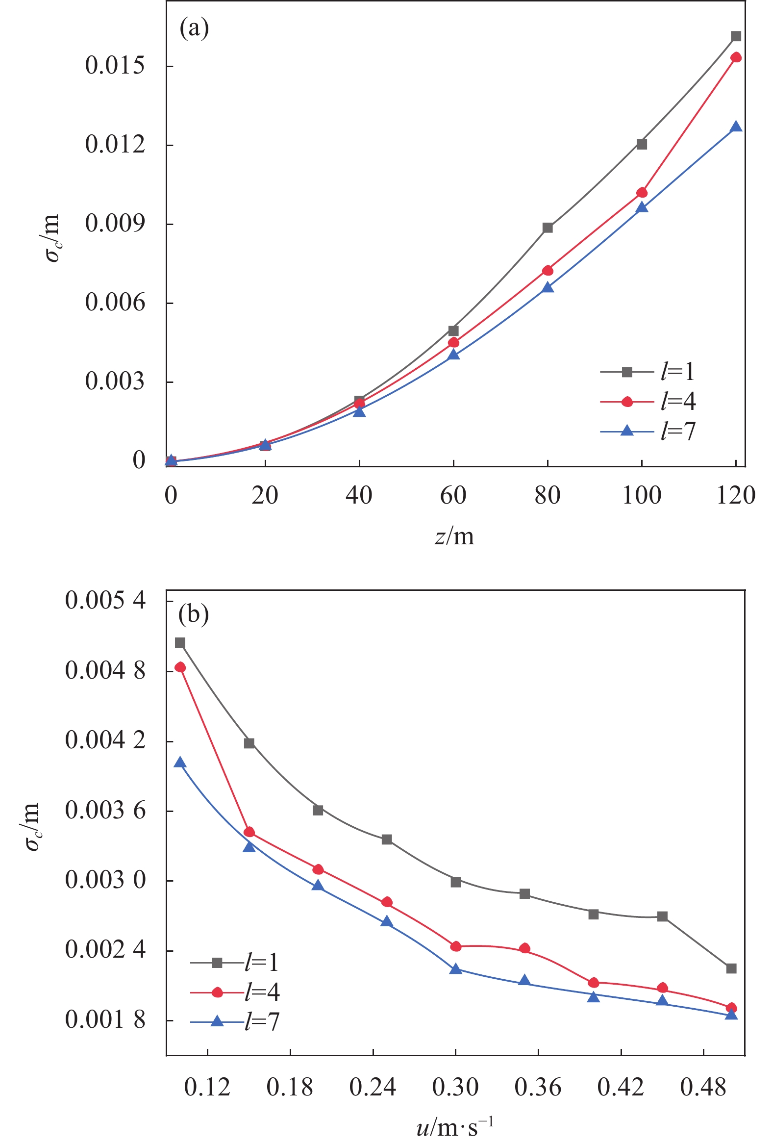
文中对涡旋光束的光斑质心取500次数学平均作为系综平均值,进而利用公式(19)得到光束漂移标准差。图6(a)、(b)分别为弱风条件下光束漂移σc。

图 6 准直高斯涡旋光束光束漂移σc。 (a)不同拓扑荷数下光束漂移与传输距离的关系; (b)不同拓扑荷数下光束漂移与水深平均流速的关系
Figure 6. The beam wander σc of collimated Gaussian vortex beam. (a) the relationship between beam wander σc and propagation distance z for the values of different the topological charge l; (b) the relationship between beam wander σc and propagation distance z for the values of different the tidal velocity of depth-averaged u
在不同拓扑荷数l时随水深平均流速u及传输距离z的变化关系。从图6可以看出,随传输距离z和水深平均流速u增大,光束漂移σc分别增大、减小,且传输距离z和水深平均流速u一定时,拓扑荷数l越大光束漂移σc越小。造成这种现象的原因是当接收机位置和天顶角ζ 固定不变时,随着传输距离z增加,发射机所处的海水深度增加,海洋湍流逐渐由温度主导变为盐度主导,且盐度主导的海洋湍流大于温度主导的海洋湍流,因此光束漂移σc增大;动能耗散率ε 随水深平均流速u的增大而增大,海洋湍流的强度减小,因此光束漂移σc减小;此外,当拓扑荷数增大时,涡旋光束的暗核增大,光束受到海洋湍流的影响减弱。
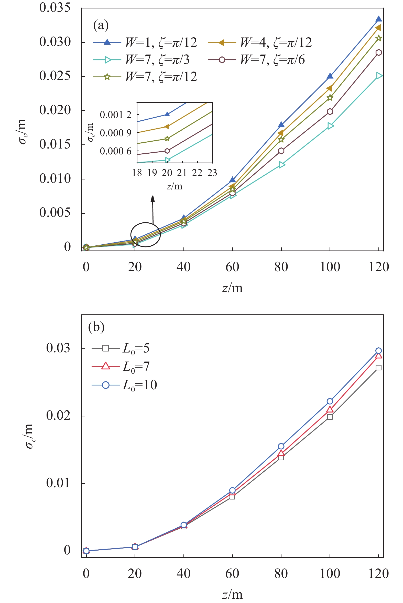
图7(a)、(b)分别为弱风条件下准直高斯涡旋光束在不同风速W和海洋湍流外尺度L0时光束漂移σc与传输距离z的变化关系。由图7可以看出,随传输距离z增大,光束漂移σc增大;从图7(a)可知,当传输距离z和天顶角ζ一定时,光束漂移σc随风速W增大而增大,当传输距离z和风速W一定时,光束漂移σc随天顶角ζ减小而增大。这种现象的物理解释为:当风速W增大时,动能耗散率ε增大,海洋湍流强度减小;当风速W和接收机位置固定时,传输距离z固定不变,天顶角ζ减小,则发射机所处位置的海水深度增加,海洋湍流逐渐由温度主导变为盐度主导且盐度主导的湍流强度大于温度主导的湍流强度,因此光束漂移σc增大;由图7(b)可知,当传输距离不变时,光束漂移σc随海洋湍流外尺度L0的增大而增大,造成这种现象的原因是随着外尺度的增大,湍流中的能量增大,此时湍流对光束漂移的影响增大。此外,由于海洋湍流外尺度不会无限大,理想情况下将海洋湍流外尺度L0取值为无穷大会高估海洋湍流引起的光束漂移效应。

图 7 准直高斯涡旋光束光束漂移σc与传输距离z的关系。 (a)不同风速W及天顶角ζ; (b)不同海洋湍流外尺度L0
Figure 7. The beam wander σc of the collimated Gaussian vortex beam versus the propagation distance z. (a) For the values of different the wind speed W and the zenith angle ζ; (b) For the values of different the outer scale of oceanic turbulence L0
-
光束在随机介质中传输时,会受到传输介质中的散射及折射会使得光束强度出现涨落,即闪烁现象。接收端光束某一点光强变化的剧烈程度可用闪烁指数表示,闪烁指数越大,光束的强度变化越剧烈。轴上闪烁指数[22]可以定义为:
$$ \sigma _I^2 = \frac{{\left\langle {{I^2}} \right\rangle }}{{{{\left\langle I \right\rangle }^2}}} - 1 $$ (20) 式中:I为光强;〈·〉是系综平均。由于相位屏是随机生成的,具有较大的随机性,文中计算了光束传输500次的数学平均值作为光束的闪烁指数。
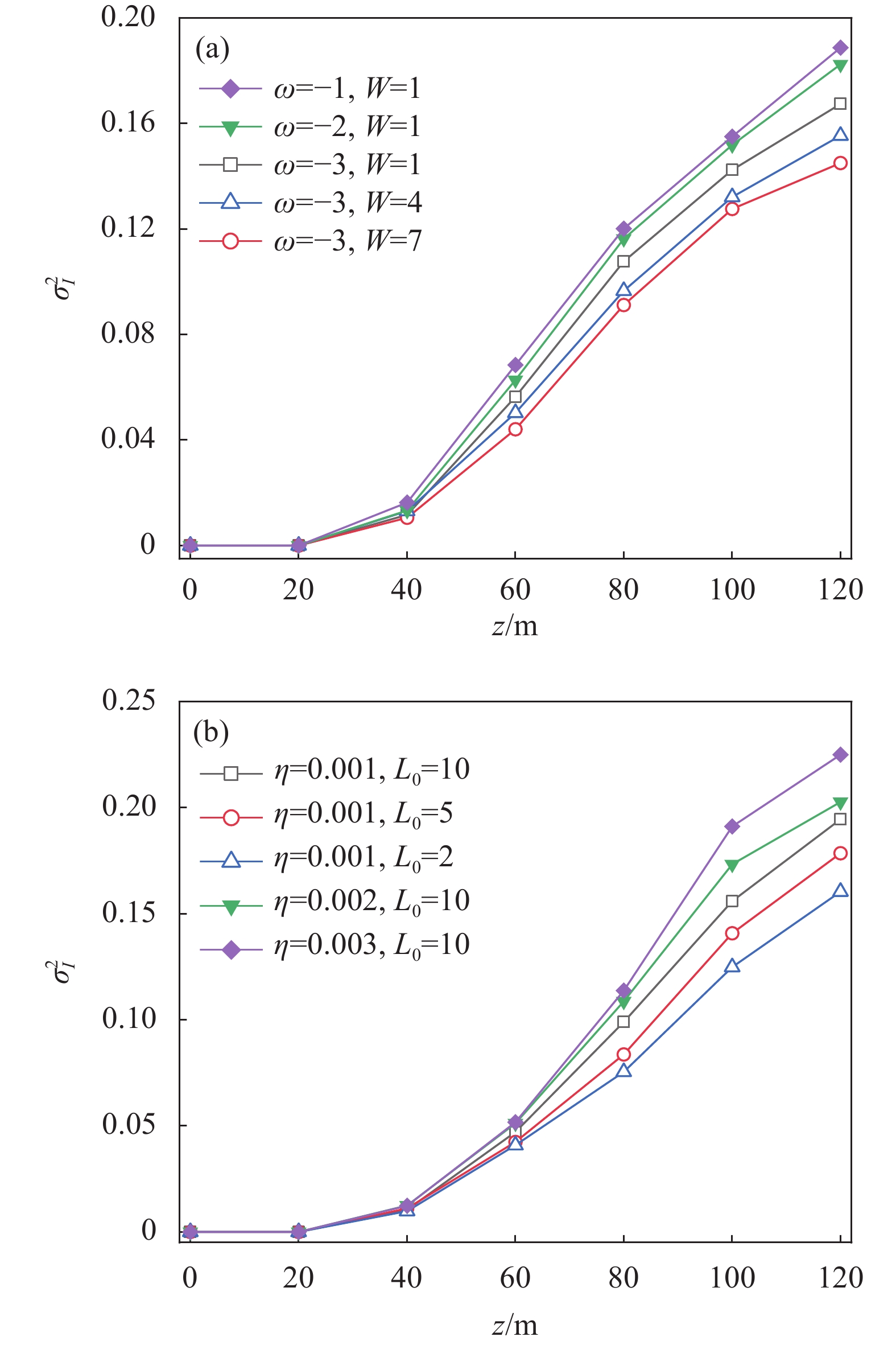
图8所示为弱风条件下轴上闪烁指数σI2在不同条件下随传输距离z的变化曲线,图8(a)为不同温度盐度贡献比 ω 及风速W时的轴上闪烁指数σI2;图8(b)为不同湍流内尺度η 及外尺度L0时的轴上闪烁指数σI2。从图8(a)中可以看出,当传输距离z一定时轴上闪烁指数σI2随着温度盐度贡献比 ω 的增大而增大,造成这种现象的原因是温度盐度贡献比ω 的取值范围为−5~0,当温度盐度贡献比ω 趋于0时湍流由盐度主导,当温度盐度贡献比ω 趋于−5时湍流由温度主导,且盐度主导的海洋湍流强度要大于温度主导的海洋湍流,所以当温度盐度贡献比ω = −1时的轴上闪烁指数σI2大于ω = −3时的轴上闪烁指数。当温度盐度贡献比ω 和传输距离z一定时,由于动能耗散率ε 随风速W的增大而增大,导致海洋湍流的强度减弱,因此轴上闪烁指数σI2随风速W的增大而减小。从图8(b)中可以看出,在弱风条件下,内尺度η对光束轴上闪烁指数的影响大于外尺度L0,且轴上闪烁指数σI2随着湍流内尺度和外尺度L0的增大而增大。原因是:随湍流内尺度η增加,湍流中的涡旋数量增大,则湍流对光束轴上闪烁指数σI2的影响增大;随着湍流外尺度L0增加,湍流中的能量增加,则湍流对轴上光束闪烁指数σI2的影响增加。

图 8 准直高斯涡旋光束轴上闪烁指数σI2与传输距离z的关系。(a) 不同风速W和温度盐度贡献比ω;(b)不同湍流内尺度η及外尺度L0
Figure 8. The on-axis scintillation index σI2 of the collimated Gaussian vortex beam versus the propagation distance z. (a) For the values of different the wind speed W and the temperature-salinity distribution ratio ω. (b) For the values of different the inner scale of oceanic turbulence η and the outer scale of oceanic turbulence L0
-
为了衡量准直高斯光束在海洋湍流上行传输链路中由湍流扰动带来的光束扩展效应,计算了准直高斯涡旋光束的长曝光光斑半径,定义为[3,22]:
$$ {W_{LE}} = \sqrt {\frac{{2 \displaystyle\iint {{r^2}I\left( {r,z} \right){d^2}r}}}{{\displaystyle\iint {I\left( {r,z} \right){d^2}r}}}} $$ (21) 经过500次统计平均,利用公式(21)计算出长曝光光斑半径。
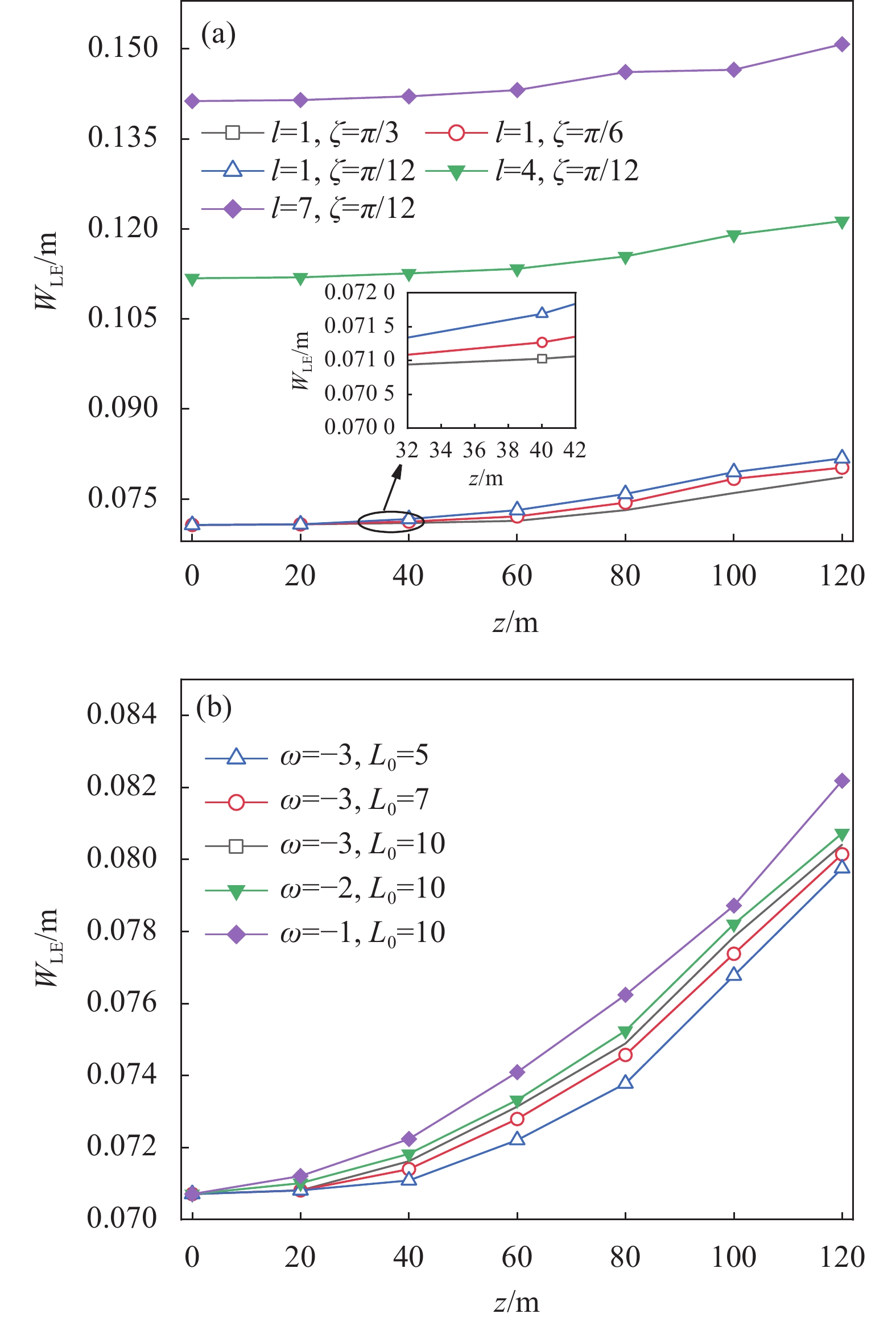
图9所示为弱风条件下准直高斯涡旋光束在拓扑荷数l、天顶角ζ、温度盐度贡献比ω和外尺度L0变化时长曝光光斑半径WLE与传输距离z的关系。从图9(a)中可以看出,长曝光光斑半径WLE随传输距离z及拓扑荷数l的增大而增大,且拓扑荷数l对长曝光光斑半径WLE的影响较大。相应的物理解释为:从图3光强分布图可知,涡旋光束的拓扑荷数l会明显影响其光斑半径,因此拓扑荷数l对长曝光光斑半径WLE的影响较大;此外,当光束传输z达到一定距离时,传输距离z对长曝光光斑半径WLE的影响开始凸显,这是因为在海洋湍流上行传输链路中,当天顶角ζ 不变时,发射机所处的海水深度随传输距离z增加而增加,此时,海洋湍流逐渐由温度主导变为盐度主导,且盐度主导的海洋湍流波动大于温度主导,因此光束传输链路受到海洋湍流影响逐渐增大。此外,当拓扑荷数l及传输距离z固定不变时,长曝光光斑半径WLE随天顶角的减小而增大,由图1的传输链路模型可知,当传输距离z固定时,天顶角ζ 越小发射机所处海水深度越深,则光束在上行传输时受到海洋湍流的影响越大。从图9(b)中可以看出,长曝光光斑半径WLE随温度盐度贡献比ω 和海洋湍流外尺度L0的增大而增大,原因是外尺度越大湍流中包含的能量越大,则湍流对长曝光光斑半径的影响越大。海洋湍流随温度盐度贡献比ω增大而增大,由于海洋的分层特性当ω=−1时海洋湍流急剧增强,因此此时长曝光光斑半径WLE快速增大。

图 9 准直高斯涡旋光长曝光光斑半径WLE与传输距离z的关系。 (a)不同拓扑荷数l及天顶角ζ ;(b)不同温度盐度贡献比ω及海洋湍流外尺度L0
Figure 9. The long-exposure beam radius WLE of the collimated Gaussian vortex beam versus the propagation distance z. (a) For the values of different the topological charge l and the zenith angle ζ; (b) For the values of different the temperature-salinity distribution ratio ω and the outer scale of oceanic turbulence L0
图10所示为弱风条件下准直高斯涡旋光束在不同水深平均流速u及风速W时长曝光光斑半径WLE与传输距离z的关系。结合图9和图10中可以看出,长曝光光斑半径WLE随传输距离z的增加而增大。从图10可以看出,当传输距离z及风速W固定时,水深平均流速u越大,光束受到的扩展效应越严重;当传输距离z及水深平均流速u不变时,长曝光光斑半径WLE随风速W的增大而减小。原因是:风速W及水深平均流速u越大,动能耗散率ε越大,导致海洋湍流减弱,光束受到湍流的影响减弱,因此光束的扩展效应减弱。

图 10 准直高斯涡旋光束的长曝光光斑半径WLE在不同水深平均流速u及风速W条件下与传输距离z的关系
Figure 10. The long-exposure beam radius WLE of the collimated Gaussian vortex beam versus the propagation distance z for the values of different the tidal velocity of depth-averaged u and the wind speed W
-
文中利用次谐波法将功率谱反演法构建的弱风条件下海洋湍流随机相位屏进行补偿并利用相位结构函数验证了相位屏的正确性,采用多相位屏法搭建斜程海洋湍流上行传输链路模型,对海洋湍流斜程路径上准直高斯涡旋光在不同影响因素下的光强及相位分布、轴上闪烁指数σI2、光束漂移σc和长曝光光斑半径WLE进行计算并分析。结果表明,当补偿阶数为7,下一次谐波采样区间数为4,设置6次谐波时,构建的海洋湍流相位屏能够更加精确地表示斜程路径下海洋湍流的统计特性;准直高斯涡旋光束的光束漂移、轴上闪烁指数及长曝光光斑半径随海洋湍流外尺度的增大而增大,理想情况下取海洋湍流外尺度为无穷大,会高估湍流对光束的影响;在海洋湍流上行传输路径中,天顶角ζ 越大,涡旋光束在传输时受到湍流的影响越小;当其他参数不变时,光束漂移σc、轴上闪烁指数σI2和长曝光光斑半径WLE主要受传输距离z影响;由于涡旋光束的本身特性,拓扑荷数对光强及相位分布和长曝光光斑半径的影响较为显著。该研究成果将为海洋湍流斜程路径下激光通信和涡旋光束的传播提供一定的理论依据。
Propagation properties of the vortex beam in the slant path of ocean turbulence under weak wind model
-
摘要: 光束在海洋介质中传输会极大地受到海洋湍流的影响。此外,涡旋光束轨道角动量的复用会极大地提高系统容量,因此研究涡旋光束在海洋湍流中的传输具有重要意义。在水平海洋湍流理论基础上,创新性地构建了斜程路径上海洋湍流相位屏模型,以相位结构函数为依据验证了海洋湍流相位屏的准确性,根据多相位屏法搭建准直高斯涡旋光束在海洋湍流中的上行传输链路模型。数值模拟并分析了不同天顶角、海洋湍流内外尺度及拓扑荷数等其他海洋湍流参数对准直高斯涡旋光束经海洋湍流上行传输的光强及相位分布、光束漂移、轴上闪烁指数和长曝光光斑半径的影响。结果表明:涡旋光束的拓扑荷数越小、天顶角越小,光束受到湍流的影响越大;在海洋湍流上行传输链路中,准直高斯涡旋光束的光束漂移、轴上闪烁指数及长曝光光斑半径随海洋湍流外尺度的增大而增大,且主要受传输距离的影响;理想情况下,取海洋湍流外尺度为无穷大,会高估湍流对光束的影响;由于涡旋光束的本身特性,拓扑荷数对光强及相位分布和长曝光光斑半径的影响也较为显著。Abstract:
Objective In recent years, with the development of underwater laser communication, laser imaging, lidar and other technologies, many scholars have carried out extensive research on the propagation of beams in ocean turbulence. Beams propagation in ocean medium is greatly affected by ocean turbulence, and the orbital angular momentum multiplexing of the vortex beam greatly increases the system capacity, thus it is of great significance to investigate the propagation of the vortex beam in ocean turbulence. Most of the previous studies have focused on the propagation of beams through horizontal ocean turbulence. However, the beam is mostly propagated through ocean turbulence in the slant path in practical applications. Methods Based on the theory of horizontal ocean turbulence, the phase screen of ocean turbulence in the slant path is generated and compensated, the correctness of ocean turbulence phase screen in the slant path is demonstrated by phase structure function. The uplink propagation link model of collimated Gaussian vortex beam in ocean turbulence is built based on the multi-phase screen method. The intensity and phase profiles, beam wander, on-axis scintillation index and long-exposure beam radius of the collimated Gaussian vortex beam in the slant path of ocean turbulence for the values of the different zenith angle, the inner scale and the outer scale of oceanic turbulence, topological charge and other ocean turbulence parameters are numerically simulated and analyzed. Results and Discussions Two-dimensional diagram of random ocean turbulence phase screen (Fig.2(a)), and the correctness of ocean turbulence phase screen in slant path is demonstrated by phase structure function (Fig.2(b)); The beam wander of collimated Gaussian vortex beam versus the propagation distance for the values of different tidal velocity of depth-averaged is simulated (Fig.6(b)); The beam wander of the collimated Gaussian vortex beam versus the propagation distance for the values of different wind speed, the zenith angle and the outer scale of oceanic turbulence is simulated (Fig.7). The on-axis scintillation index of the collimated Gaussian vortex beam versus the propagation distance for the values of different inner scale and the outer scale of oceanic turbulence is simulated (Fig.8(b)). Conclusions The correctness of ocean turbulence phase screen in slant path is demonstrated by phase structure function. The uplink propagation link model of ocean turbulence is simulated by multi-phase screen method. The results show that the smaller the topological charges and the larger the inner scale and the outer scale of oceanic turbulence the vortex beam, the greater the influence of turbulence on the beam is; The beam wander, the on-axis scintillation index and the long-exposure beam radius of collimated Gaussian vortex beam increase with the increase of the outer scale of ocean turbulence. Ideally, the outer scale of ocean turbulence is taken as infinity to overestimate the effect of ocean turbulence on the beam. The beam wander and the on-axis scintillation index are mainly affected by the propagation distance in the uplink propagation of ocean turbulence; Moreover, because of the characteristics of the vortex beam, the topological charges and the long-exposure beam radius have significant effects on the intensity and phase profiles and the long-exposure beam radius. -
图 1 光束通过海洋湍流相位屏上行传输链路模型示意图
Figure 1. Schematic diagram of the beam through phase screen in uplink transmission channel model of ocean turbulence
图 2 海洋湍流随机相位屏二维图及相位结构函数验证图。 (a)相位屏二维图; (b)相位结构函数验证图
Figure 2. Two-dimensional diagram of random ocean turbulence. (a) Phase screen; (b) Phase structure function curves
图 3 准直高斯涡旋光束在斜程海洋湍流中不同传输距离处的光斑强度分布情况
Figure 3. Intensity profiles of collimated Gaussian vortex beam at different propagation distance in ocean turbulence of slant path
图 4 准直高斯涡旋光束在不同拓扑荷数时相位随传输距离变化的相位分布图
Figure 4. Phase profile of collimated Gaussian vortex beam with different topological charges as a function of propagation distance
图 6 准直高斯涡旋光束光束漂移σc。 (a)不同拓扑荷数下光束漂移与传输距离的关系; (b)不同拓扑荷数下光束漂移与水深平均流速的关系
Figure 6. The beam wander σc of collimated Gaussian vortex beam. (a) the relationship between beam wander σc and propagation distance z for the values of different the topological charge l; (b) the relationship between beam wander σc and propagation distance z for the values of different the tidal velocity of depth-averaged u
图 7 准直高斯涡旋光束光束漂移σc与传输距离z的关系。 (a)不同风速W及天顶角ζ; (b)不同海洋湍流外尺度L0
Figure 7. The beam wander σc of the collimated Gaussian vortex beam versus the propagation distance z. (a) For the values of different the wind speed W and the zenith angle ζ; (b) For the values of different the outer scale of oceanic turbulence L0
图 8 准直高斯涡旋光束轴上闪烁指数σI2与传输距离z的关系。(a) 不同风速W和温度盐度贡献比ω;(b)不同湍流内尺度η及外尺度L0
Figure 8. The on-axis scintillation index σI2 of the collimated Gaussian vortex beam versus the propagation distance z. (a) For the values of different the wind speed W and the temperature-salinity distribution ratio ω. (b) For the values of different the inner scale of oceanic turbulence η and the outer scale of oceanic turbulence L0
图 9 准直高斯涡旋光长曝光光斑半径WLE与传输距离z的关系。 (a)不同拓扑荷数l及天顶角ζ ;(b)不同温度盐度贡献比ω及海洋湍流外尺度L0
Figure 9. The long-exposure beam radius WLE of the collimated Gaussian vortex beam versus the propagation distance z. (a) For the values of different the topological charge l and the zenith angle ζ; (b) For the values of different the temperature-salinity distribution ratio ω and the outer scale of oceanic turbulence L0
-
[1] Ijeh I C, Khalighi M A, Elamassie M, et al. Outage probability analysis of a vertical underwater wireless optical link subject to oceanic turbulence and pointing errors [J]. Journal of Optical Communications and Networking, 2022, 14(6): 439-453. doi: 10.1364/JOCN.454191 [2] 张凤, 张明明, 胡友友等. Ince-Gaussian光束在海洋湍流中的传输特性[J]. 应用激光, 2022, 42(11): 92-98. Zhang Feng, Zhang Mingming, Hu Youyou, et al. Propagation properties of ince-gaussian beams in oceanic turbulence [J]. Applied Laser, 2022, 42(11): 92-98. (in Chinese) [3] 杨祎, 聂欢, 王晓波等. 海洋湍流外尺度对高斯光束传输特性的影响[J]. 光子学报, 2023, 52(04): 114-126. Yang Yi, Nie Huan, Wang Xiaobo, et al. Influence of outer scale of ocean turbulence on propagation characteristics of gaussian beams [J]. Acta Photonica Sinica, 2023, 52(4): 0401002. (in Chinese) [4] 张艺伟, 王明军. 反常涡旋光束在分层海洋湍流中的光强和相位特性研究[J]. 激光杂志, 2022, 43(06): 13-18. Zhang Yiwei, Wang Mingjun. Intensity and phase characteristics of anomalous vortex beams in stratified ocean turbulence [J]. Laser Journal, 2022, 43(6): 13-18. (in Chinese) [5] Pompili D, Akyildiz I F. Overview of networking protocols for underwater wireless communications [J]. IEEE Communications Magazine, 2009, 47(1): 97-102. doi: 10.1109/MCOM.2009.4752684 [6] Mcglamery B L. Computer simulation studies compensation of turbulence degraded images [C]//Pacific Grove, Image processing, SPIE, 1976, 74: 225-233. [7] Noll R J. Zernike polynomials and atmospheric turbulence [J]. Journal of the Optical Society of America, 1976, 66(3): 207-211. doi: 10.1364/JOSA.66.000207 [8] Perez D G, Zunino L, Garavaglia M. Modeling turbulent wave-front phase as a fractional Brownian motion: a new approach [J]. Journal of the Optical Society of America A, 2004, 21(10): 1962-1969. doi: 10.1364/JOSAA.21.001962 [9] Fleck J A, Morris J R, Feit M D. Time-dependent propagation of high energy laser beams through the atmosphere [J]. Applied Physics, 1976, 10(2): 129-160. doi: 10.1007/BF00896333 [10] Lane R G, Glindemann A, Dainty J C. Simulation of a Kolmogorov phase screen [J]. Waves in Random Media, 1992, 2(3): 209-224. doi: 10.1088/0959-7174/2/3/003 [11] Farwell N H, Korotkova O. Multiple phase-screen simulation of oceanic beam propagation[C]//Laser communication and propagation through the atmosphere and oceans III, SPIE, 2014, 9224: 374-380. [12] 杨天星, 赵生妹. 海洋湍流随机相位屏模型[J]. 光学学报, 2017, 37(12): 9-14. Yang Tianxing, Zhao Shengmei. Random phase screen model of ocean turbulence [J]. Acta Optica Sinica, 2017, 37(12): 9-14. (in Chinese) [13] 牛超君, 卢芳, 韩香娥. 相位屏法模拟高斯阵列光束海洋湍流传输特性[J]. 光学学报, 2018, 38(06): 31-36. Niu Chaojun, Lu Fang, Han Xiang’e. Propagation properties of gaussian array beams transmitted in oceanic turbulence simulated by phase screen method [J]. Acta Optica Sinica, 2018, 38(6): 31-36. (in Chinese) [14] Pan S, Wang L, Wang W, et al. An effective way for simulating oceanic turbulence channel on the beam carrying orbital angular momentum [J]. Scientific Reports, 2019, 9(1): 1-8. doi: 10.1038/s41598-018-37186-2 [15] 张凯宁, 刘永欣, 蒲继雄. 涡旋光束在海洋湍流中传输的闪烁因子[J]. 中国激光, 2019, 46(07): 247-252. Zhang Kaining, Liu Yongxin, Pu Jixiong. Scintillation index of vortex beams propagating in oceanic turbulence [J]. Chinese Journal of Lasers, 2019, 46(7): 247-252. (in Chinese) [16] Li Ye, Li Baolong, Jiang Haolin. Displacements of a spatially limited light beam in the slant path of oceanic turbulence [J]. Optics Express, 2022, 30(14): 24232-24244. doi: 10.1364/OE.461026 [17] Pu Huan, Ji Xiaoling. Oceanic turbulence effects on long-exposure and short-exposure imaging [J]. Journal of Optics, 2016, 18(10): 105704. doi: 10.1088/2040-8978/18/10/105704 [18] Feistel, R, Nausch, G, Hangen, E. Unusual Baltic inflow activity in 2002-2003 and varying deep-water properties [J]. Oceanologia, 2006, 48(S): 21-35. [19] Chhabra S, Paue J, Ramaprakash A N, et al. Generalized approach to compensate for low-and high-frequency errors in fast Fourier transform-based phase screen simulations [J]. Journal of Astronomical Telescopes, Instruments, and Systems, 2021, 7(2): 025007. [20] Luo Chuankai, Lu Fang, Han Xiang’e. Propagation and evolution of rectangular vortex beam array through atmospheric turbulence [J]. Optik, 2020, 218: 164913. doi: 10.1016/j.ijleo.2020.164913 [21] Wang Mingjun, Cheng Qun, Li Jianqing, et al. Transmission characteristics of blue-green vortex beams in the lower atmosphere-upper ocean link [J]. Journal of Quantitative Spectroscopy and Radiative Transfer, 2022, 286: 108205. doi: 10.1016/j.jqsrt.2022.108205 [22] Andrews L C, Phillips R L. Laser Beam Propagation Through Random Media[M]. 2nd ed. Bellingham: Laser Beam Propagation Through Random Media, 2005. [23] Lu Lu, Ji Xiaoling, Baykal Y. Wave structure function and spatial coherence radius of plane and spherical waves propagating through oceanic turbulence [J]. Optics Express, 2014, 22(22): 27112. doi: 10.1364/OE.22.027112 [24] 吴彤, 季小玲, 李晓庆等. 海洋湍流中光波特征参量和短期光束扩展的研究[J]. 物理学报, 2018, 67(22): 271-279. Wu Tong, Ji Xiaoling, Li Xiaoqing, et al. Characteristic parameters of optical wave and short-term beam spreading in oceanic turbulence [J]. Acta Physica Sinica, 2018, 67(22): 271-279. (in Chinese) [25] Fried D L. Optical resolution through a randomly inhomogeneous medium for very long and very short exposures [J]. Journal of the Optical Society of America, 1966, 56(10): 1372-1379. doi: 10.1364/JOSA.56.001372 [26] Li Ye, Zhang Yixin, Zhu Yun. Oceanic spectrum of unstable stratification turbulence with outer scale and scintillation index of Gaussian-beam wave [J]. Optics Express, 2019, 27(5): 7656-7672. doi: 10.1364/OE.27.007656 -

 点击查看大图

计量
- 文章访问数: 109
- HTML全文浏览量: 36
- PDF下载量: 33
- 被引次数: 0

