Mixed-precision quantization for neural networks based on error limit (Invited)

近年来，基于卷积神经网络（Convolutional Neural Networks, CNN）的深度学习方法受到了学术界和工业界的关注，在目标分类、目标检测等方面得到了广泛的应用，已经成为各种计算机视觉任务的主流方法。随着数据集规模的扩大、硬件设备的发展，可处理卷积神经网络模型的层数也在不断增加，例如，从AlexNet^[1]、VGGNet^[2]、GoogleNet到ResNet^[3]，ILSVRC挑战赛的冠军模型已经从8层提升到100多层。随着层数的加深，模型参数规模与计算强度也随之增大增强。一个50层的残差网络有超过2550万个参数，模型推理时计算量更是达到4 GFLOP以上。如此庞杂的参数量与数据量为其在带宽与存储受限的边缘设备上部署平添了诸多问题。主要包括：

（1）模型大小的限制：深度学习卷积网络模型中数百万个可训练参数成就了其强大的检测能力。例如，存储一个经过训练的语义分割DeepLabV3+模型会占用超过100 MB内存空间，这对硬件设备是一个巨大的资源负担。

（2）运行内存：在推理过程中，CNN的卷积操作中间变量会占用更多的内存空间，普通硬件设备难以支撑。

（3）计算用时：在对高分辨率图像进行密集卷积操作时，硬件设备往往延时较高，难以在较低功耗下实现实时的结果预测。

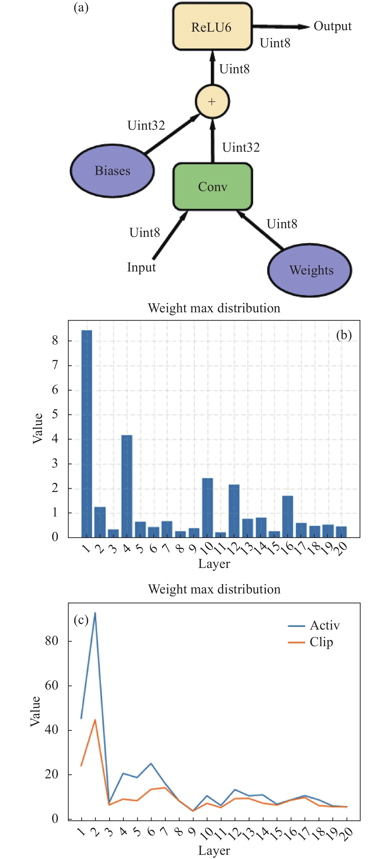
参数量化通过减少神经网络参数值所需的数据位宽来压缩原始网络。且量化后，低精度定点乘累加运算（Multiply Accumulate，MAC）可以替代浮点运算以降低资源开销与硬件能耗。Vanhoucke等人^[4]的研究表明，8位推理运算能够在提升速度的同时保证最小的模型精度损失。目前主流的量化方法大多数采用统一精度量化，如统一16位量化方法^[5]、谷歌8位量化方法^[6]，将网络模型各层的权重和激活数据量化至相同的位宽。但不同卷积层中参数的分布范围和冗余度都不相同，如图1（b）中展示了YOLOV5 s网络前20层中的权重参数分布。可以看出，各层的权重最值分布有较大的差异，第1层的权重最大值约为第3层的25倍。因此一些研究者提出了差异位宽分布的混合精度量化方法。如零样本量化框架（a novel zero shot quantization framework, ZeroQ）方法^[7]、强化学习量化策略搜索方法^[8-9]等，通过奖励函数设置不同卷积层的量化位宽，训练得到最优分配策略。

Figure 1.  (a) Photograph of deep learning convolutional 8-bit quantization procession^[6]; (b) The distribution trend of the most valued weights in the first 20 layers of the YOLOV5 s network; (c) Distribution of activation maximum and cutoff value during network quantization in YOLOV5 s

文中对比了不同量化方法在VOC2007数据集上的表现，选择合适的量化方法，通过对各层的放缩因子进行统一等比限制，得到了合适的网络模型分层量化方法，并依据该方法对权重和激活值进行混合截断量化，取得了更高的准确率。文中的工作包含以下方面：

(1) 通过对比移位量化形式与乘积量化形式、无截断量化方法与基于均方误差的截断量化方法，选择最优方法作为文中的实现方法；

(2) 提出基于误差限制的量化搜索策略，不同于强化学习或策略搜索等方法，文中方法具有更低的复杂度与更高的普遍性，可快速获取分层量化策略；

(3) 根据混合精度分层量化策略对YOLOV5 s网络中不同卷积层数据进行混合截断量化，并使用VOC2007数据集进行对比实验；

(4) 在COCO数据集和VOC2011数据集上使用YOLOV5 s网络对混合精度量化方法进行测试。

目前，深度学习神经网络的主流压缩和加速方法主要有两类：模型剪枝、参数量化^[10]。

模型剪枝是深度学习神经网络模型中应用最为广泛的压缩与加速方法，基本思想是通过对训练后的CNN模型进行稀疏化操作，剪除冗余的、信息量较少的参数值，达到压缩模型大小的目的。在2015年，Chen等人^[11]提出了HashedNets模型，引入哈希函数并根据参数间汉明距离重组权重，实现参数共享，是典型的非结构化剪枝方法。然而，非结构化剪枝在计算过程中引入稀疏矩阵造成内存获取的不规则性，影响硬件工作效率，进而降低运算速度。2017年，Liu等人^[12]提出一种通道级别结构化剪枝方法，向存在于每个卷积层的批量标准化（Batch Normalization）中的缩放因子添加稀疏正则限制，通过批量标准化中超参数γ的大小对卷积通道进行剪除，再通过微调恢复精度，有效降低了网络复杂度。2020年，徐等人^[13]为所有卷积层中的卷积核数量乘以缩小因子α以压缩网络，有效地降低了冗余参数，同时压缩后的计算量减少了α倍。Lin等人^[14]提出一种基于特征图矩阵秩的滤波器剪枝方法，剪除低秩特征图的滤波器，在ResNet-110上缩小了58.2%的计算量，精度仅损失0.14%。He等人^[15]提出了一种滤波器剪枝准则（Learning Filter Pruning Criteria, LFPC）指导剪枝，该方法能够考虑到网络中所有层的协同作用，自适应为不同卷积层选择适合自己的剪枝规则。

量化是卷积神经网络模型压缩移植的主要实现方法。2015年，Han等人^[16]引用一个三阶段的管道流程—网络权重剪枝、训练量化网络、哈夫曼编码，将神经网络的存储需求压缩到原来的$ \dfrac{1}{35}\sim\dfrac{1}{49} $。2017年，谷歌提出一种非对称量化方法^[6]，如图1（a）中所示，将权重和激活都量化到8位整数，并在训练阶段添加量化训练框架以模拟量化运算带来的误差，能够最大限度地减少真实模型上量化带来的精度损失。2019年，Gong等人^[17]提出了Differentia-ble Soft Quantization(DSQ)方法构建可微分的软量化函数，使得量化参数也可以跟随神经网络一起训练学习。2020年，Zhu等人^[18]在将网络参数量化到8 bit的同时，引入了误差敏感的学习率调节方法，并且对量化造成的精度损失问题提出了方向自适应的梯度阶段处理方法。

统一精度量化将神经网络中所有层量化到固定的位宽，而混合精度量化为不同层分配不同的位宽。事实上，卷积神经网络各层的权重最大值分布是不同的，因此，2019年，Wang等人^[8]提出基于硬件感知的混合精度自动量化方法方法，将寻找目标网络混合量化策略的问题建模为强化学习问题，通过深度确定性策略梯度（deep deterministic policy gradient, DDPG）算法自动搜索最佳量化策略。Huang等人^[9]优化了强化学习中的奖励函数设置，使得搜索出的量化策略够在更小的模型下仍有较高的准确率。

人工搜索合适的分层量化策略是非常困难的。如经典的YOLOV3_TINY^[19]算法，拥有13个卷积层，可能的量化策略就有$ {8}^{13} $种，仅靠人工搜索最佳策略是几乎不可能完成的任务。目前的主流的剪枝方法和量化搜索策略依赖强化学习(reinforcement learning)或进化算法(evolutionary algorithm-m），需要较长的搜索阶段才能收敛，且当对不同的数据集以及压缩率进行实验时，强化学习方法都需要进行重新调参和训练以获得最终结果。文中通过对量化舍入误差分析，提出基于误差限制的混合精度量化方法，相比于强化学习方法，文中拥有更低的时间复杂度与更高的普遍性；相比于全层统一精度量化方法，文中在同样压缩率下拥有更高的精度。

量化将浮点数转换为定点数进行运算，在推理过程中只使用整数，因此对于硬件实现更加友好高效。文中在表1所示的两种量化方法中选择，其中,$ round\left(x\right) $函数为四舍五入，乘积运算因子$ s $定义为$ s={w}_{max}/\left({2}^{bi-1}-1\right) $，代表着量化运算前后的缩放尺度；$ fl={b}_{i}-1- ⌈{\mathrm{log}}_{2}{w}_{max}⌉ $为量化的移位因子，代表量化运算的移位步长。移位量化方法缩小了量化运算带来的功耗损失，在提高运算效率的同时增大了精度损失。使用YOLOV5 s网络在VOC2007数据集上分别对两种方法进行了测试，结果如表2所示。乘积量化方法在低位宽量化时相较于移位量化方法整体拥有更高的精度，随着量化位宽的降低，两种方法的精度损失逐步增大，移位量化方法的精度损失下降更快，乘积量化方法在7位量化时仍有不错的精度。

硬件设备一般存储卷积神经网络中的权重和偏置等信息，在观察网络中各层权重分布时，有一些离散值的存在，数量很小，但影响该层权重的最大值，增加了权重分布范围，进而影响了量化后网络的准确率。因此，对权重数据先截断再量化，可以减少量化带来的精度损失。如图1（c）中所示，YOLOV5 s前20层中实际采用的截断值约为原始最大值的1/2。文中采用截断操作优化乘积运算的量化方法，具体来说，该方法逐层将权值截断至$ \left[-c,c\right] $的范围，后将其量化至$ {b}_{i} $位。量化方法为：

式中：$ \mathrm{c}\mathrm{l}\mathrm{a}\mathrm{m}\mathrm{p}\left(w,c\right) $表示将权值$ w $截断到$ \left[-c,c\right] $的范围；$ {b}_{i} $为第i层量化位宽。截断值c的选择如下：

式中：$ {d}_{MSE} $表示原始权值分布和量化模拟后的权重分布之间的均方误差。

文中在YOLOV5 s网络对VOC2007数据集使用截断方法前后的性能进行了测试对比，结果如表3所示，其中，MAX代表最大值量化，MSE表示基于均方误差（mean squared error, MSE）的截断量化方法。可以看出，截断方法能够有效控制量化误差，在各个量化位宽，相较于无截断方法均有一定的精度提升，且位宽越低，性能对比越明显，当量化位宽为5 bit和6 bit时，采用MSE截断量化方法比无截断量化方法性能分别提升了27.7%和22.3%，说明基于均方误差的量化方法能有效恢复检测精度。

量化过程中的误差主要来自于两个方面：取整损失与截断损失。截断操作的引入可以缩小量化区间，减少量化过程中的取整损失。在此分析软件端模拟量化过程中的取整损失。

输入量化操作：

权重量化操作：

偏置量化操作：

激活量化操作为：

由于四舍五入取整操作带来的损失在0.5以内，因此输入量化、权重量化以及激活量化操作带来的误差均在$ 0.5\times \mathrm{s}\mathrm{c}\mathrm{a}\mathrm{l}\mathrm{e} $范围内。且与$ \mathrm{s}\mathrm{c}\mathrm{a}\mathrm{l}\mathrm{e} $大小成正相关。文中认为，每一层对最终结果的影响都是相同的，因此，笔者课题组可以选择一种误差限制的量化策略，通过对卷积层的放缩因子$ \mathrm{s}\mathrm{c}\mathrm{a}\mathrm{l}\mathrm{e} $的大小进行限制，得到不同卷积层的量化精度。使用γ作为卷积层的误差限制参数，初始时设置所有卷积层的量化位宽为8，如果放缩因子$ \mathrm{s}\mathrm{c}\mathrm{a}\mathrm{l}\mathrm{e} $小于γ，则该层位宽减1,直至该层放缩因子$ \mathrm{s}\mathrm{c}\mathrm{a}\mathrm{l}\mathrm{e} $超过γ。整体流程如图2所示。

Figure 2.  Framework of network hierarchical policy methodology

文中设计循环计算获得最佳γ，初始位宽设置为8，逐层推理并调整位宽大小，从而确定最佳位宽策略。由于卷积层中最大值出现在激活部分，因此使用激活部分放缩因子$ \mathrm{s}\mathrm{c}\mathrm{a}\mathrm{l}\mathrm{e} $与γ进行对比，如果$ \mathrm{s}\mathrm{c}\mathrm{a}\mathrm{l}\mathrm{e} $小于γ，则该层位宽减1，直至该层放缩因子超过γ，进入下一卷积层。

笔者课题组在YOLOV5 s训练VOC2007数据集的量化方法探索中，测试了不同γ值对于量化结果的影响，如表4所示。γ可设置在$ \left[\mathrm{0.08,0.25}\right] $之间，在最佳点之前，网络精度随着压缩率的增加在不断波动，达到最佳点之后，随着压缩率的增加，网络精度整体呈现

下降趋势，相较于表3，VOC数据集统一量化到7位和5位的精度分别为76%和31.7%，混合量化到6.49位和5.07位的精度分别为79.6%和63.3%。混合精度量化方法均能在更小的模型中达到更高的检测精度。

由于大部分网络的激活函数都使用ReLU函数，因此每一层的输出函数的分布范围为$ \left[0,c\right] $。对于ReLU激活函数的缩放因子s，文中定义为$ {s}=c/({2}^{bi}-1) $，对于Leaky ReLU、SiLU等值域涉及负数的激活函数，文中使用${s}=c/({2}^{bi-1}-1)$作为量化放缩因子。

部分卷积神经网络拥有链接模块与残差模块。链接模块用于在指定维度链接两个张量，残差模块拥有张量相加操作。

链接操作：

相加操作：

文中在神经网络中涉及多个张量之间的操作时，对多个张量采用统一的缩放因子与量化位宽。即：

为了验证文中的方法，笔者课题组在搭载显存为24 GB的Geforce RTX 3090的服务器上进行实验，系统环境为Ubuntu16.04，Pytorch版本为1.10.1，Torchvision版本为0.4.2，Python版本为3.6.0，网络学习率为$ {10}^{-4} $，YOLOV5网络结构使用已有的Pytorch实现方法与提供的YOLOV5 s.pt预训练模型。

YOLOV5网络是目前单阶段目标检测网络中性能最好的网络之一，文中在COCO数据集和VOC2011数据集上对统一量化方法与基于误差限制的混合截断量化方法进行了对比测试，如表5所示。

在COCO数据集，与统一6位量化(模型为5.45 MB)相比，文中的方法在5.05 MB时拥有更高的精度，性能分别提升了3.3% (mAP@0.5)和2.1% (mAP@0.5-0.95)，与统一5位量化相比，文中在相似的模型大小下性能分别提升了6% (mAP@0.5)和4.5% (mAP@0.5-0.95)。

在VOC2011数据集，相比全精度模型，文中的方法将模型压缩到5.05 MB的同时mAP@0.5提升了3.1%，部分图片的检测效果有所提升；与统一精度量化方法相比，文中的方法在相似的模型大小(统一5位量化与平均5位量化)下性能分别提升了24.9%(mAP@0.5)和16.1% (mAP@0.5-0.95)。

整体上看，随着量化位宽的降低，统一精度量化方法和混合精度量化方法带来的精度损失都在逐步增加，但文中的方法能够将量化误差平均分配在各个卷积层，减少了部分层误差较大情况的出现，因此精度下降较缓，整体上相对于统一精度量化方法拥有更高的精度。表6展示了VOC2011数据集采用不同方法进行检测的不同类别的精度，可以看出，混合精度量化方法与统一精度量化方法相比，Dog类别精度有所下降，Bird、Chair、Sheep、Train类别精度相同，Aeroplane、Bicycle、Boat、Bottle、Person、Tvmonitor类别精度均有所上升。图3展示了YOLOV5 s对COCO数据集采用不同量化方法的检测结果，其中，图3（a）为训练真值，标识出了全部待检测目标；图3（b）为全精度检测结果；图3（c）为采用文中的方法进行混合6位量化的检测结果；图3（d）为统一6位量化方法的检测结果。从图中可以看出，当γ为0.09时，模型压缩到5.43 MB，即平均6位量化，对目标图像的检测效果与原始网络相当，而统一6位量化方法会丢失一些小目标与背景模糊物体的检测框。如第一张图片丢失了小目标背包的检测框，第二张图片丢失了桌子上的部分小目标检测框，对被遮挡人物的检测也有所损失。第三张图片中则损失了两辆背景模糊的车辆检测框。在第二张图片中，原始网络对于中间人物的检测出现精度损失，而6位混合量化方法恢复了人物的检测损失。

Figure 3.  Example of COCO dataset detection results

文中深入探讨了不同量化形式与量化方法对于卷积神经网络结果的影响，最终选择基于均方误差的截断方法作为文中的量化方法，同时，通过对网络量化过程中的舍入误差分析，提出基于误差限制的深度学习分层量化策略，采用误差限制因子γ对卷积层误差参数进行等比限制，得到不同卷积层的量化精度，并据此对网络参数进行混合截断量化。最终使用YOLOV5 s网络在COCO数据集和VOC数据集上进行测试并验证，与统一精度量化相比，YOLOV5 s网络混合量化到5位精度分别提升了6%和24.9%。目前，已通过算法实现并验证了混合精度量化方法在目标检测领域的应用，下一步工作将考虑对比尝试更多的量化方法、优化分层策略并在硬件端实现目标检测网络的混合位宽推理。