Internal parameter calibration method of line-scan camera based on 2.5D calibration fan

相机标定是视觉测量的基本工作，需预先建立物方世界坐标与像方平面坐标之间的几何模型，利用特征点对求解模型参数^[1]。常用视觉测量相机包括面阵相机和线阵相机，面阵相机标定的研究已经比较成熟^[2]，但线阵相机通常仅对一维空间成像，所以面阵相机的标定方法无法直接采用，且关于线阵相机内参数标定的研究文献相对较少^[3−4]。

目前线阵相机内参数的标定方法一般从设计标靶、参数标定模型、解算方法入手^[5]，总体可分为静态标定和动态标定两类，标定目标包括2D和3D两种。静态标定方面，Horaud等人最早开展关于线阵相机标定的研究，根据线阵相机的静态成像模型提出了一种基于交比不变性的标定方法。该方法计算相对简单，但其参数标定精度受移动平台的位移精度影响，且未顾及镜头非线性畸变的影响^[6]。为了避免使用高精度的移动平台，Luna的方法使用了3D标定物，但该方法对3D标定物的制造精度要求较高，特征线数量有限且提取困难^[7]。Li等人借鉴了张正友的面阵相机标定方法，克服了上述问题，但需要额外的面阵相机进行辅助标定，且标定精度取决于面阵相机的标定精度和测量精度，这使得标定过程更加复杂^[8]。Song等人设计了一种基于八卦图形的三维标定物，理论上提高了标定精度，但该标定物需要高额成本以保证制造精度，且特征提取过程较为复杂^[9]。Liao等人设计了一款3D空心条纹标定物，虽解决了偏心误差的问题，但标定物制造难度大、特征点数量少，仅限实验环境下使用^[10]。关于动态标定的研究，Draréni等人首先提出了一种基于二维靶标面的动态标定方法，该方法特征点提取方便且标定精度较高，但该方法计算复杂度较高，并要求标定物在特定的方向上运动^[11]。Hui等人先后提出了使用2D标定物和3D标定物的标定方法，不仅考虑了镜头畸变的影响而且解除了相机只能在特定方向移动的限制，但需建立复杂的动态标定模型，难以满足现场环境下标定^[12−13]。表1对不同标定方法进行了统计和对比^[5]。总体上，3D标定物制作难度和成本比2D标定物更高，但标定操作的复杂度更低；动态标定比静态标定的方法复杂，但高复杂性的算法往往可以换取较低的重投影误差。此外，为获得高精度的标定结果，可增加特征点数量，且标定模型应顾及镜头畸变的影响^[5]。

现有方法均需在实验环境下完成线阵相机内参数标定，对已投入运行的集成设备中线阵相机很难完成内参数的定期检校。针对以上问题和实际需要，提出一种基于2.5D标定扇的线阵相机标定方法。首先，受中国传统折扇的启发，设计一款2.5D的简易标定扇，解决特征点数量少和易丢失的问题；其次，在此基础上构建不受线阵相机运动方向严格限制的参数标定模型，可解算出相机与靶面不平行、不垂直的小角度误差，并顾及了镜头畸变参数；然后，利用特征点对建立标定方程组，将模型线性化方程的解作为参数初值，再基于改进Levenberg-Marquardt (L-M)算法加速优化标定参数的求解过程。

2.5D是一种介于2D和3D之间的表现形式，在平面上模拟3D效果。2.5D标靶既有3D立体测量特性，又有2D制作简单、成本低的优点。现有2D或3D标定物常以黑白线条、多边形图案等为特征，特征数量较少且缺乏关联性，部分标靶制作难度大、成本高，不便于携带和存放。在文献[18]的基础上，为获得相同基准且不同角度的多组特征点，设计了一款2.5D的标定扇，将特征点均匀布设在每根扇骨上，利用扇骨间夹角获得不同位置的多组特征点。每根扇骨的尺寸如图1(a)所示；图1(b)为标定扇立体图与直径1 mm的特征圆，其中有13根扇骨，相邻扇骨间夹角为3°，每个扇骨面上12个特征圆；图1(c)中以第7根扇骨面为$ O - XZ $面建立右手坐标系，$ \theta $为扇骨面与$ O - XZ $面的夹角；将各面上的特征亮圆正投影到$ O - XZ $面得到标定扇靶面，如图1(d)所示；将其1∶1打印在250 g铜版纸上，并平铺于光学平面上作为标靶，如图1(e)所示。

Figure 1.  Design of the calibration fan

上述设计的2.5D标定扇具有2D标靶低成本、高精度的优点，也兼具3D标靶获取不同位置特征数据的可行性。需说明的是，靶面上特征点数量虽多（可继续增加），但其呈规律性分布，因此便于与像点配对。

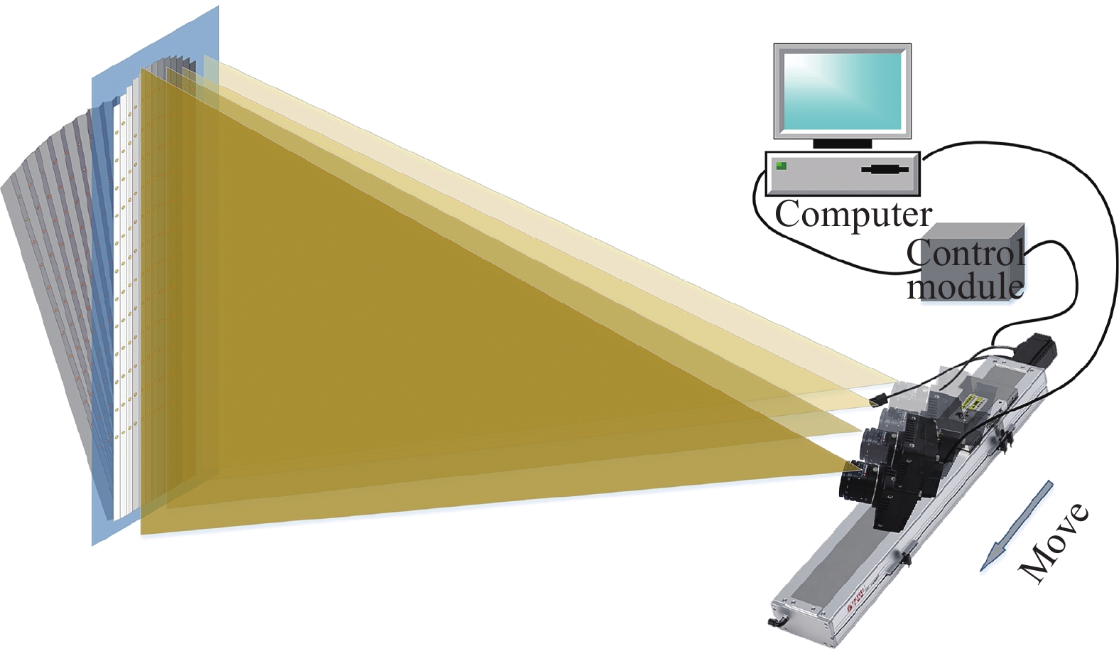
线阵相机仅包含一维成像单元，沿像元排列方向满足中心投影特征。将2.5D标定扇近似平行的放置在相机前方，相机随导轨移动采集标靶图像，如图2。在此基础上，图3描绘了特征点在图像坐标系$ (Y) $、相机坐标系$ ({X_c},{Y_c}) $、世界坐标系$ ({X_w},{Y_w},{Z_w}) $中的成像原理。$ {Y_w} $轴与$ {O_c} - {X_c}{Y_c} $共面，沿标定扇的靶面向上，$ {Z_w} $轴平行于运动方向，$ {O_w} $为过单根扇骨上所有圆心的直线与扇骨底端的交点，$ ({D_x},{D_y}) $为$ {O_w} $在相机坐标系$ ({X_c},{Y_c}) $中的坐标。$ P $为立体扇骨面的特征圆，$ {O_w}P = Y $。$ P' $为$ P $在标定扇靶面上的投影点，$ \theta $为$ P $点所在扇骨面与靶面的夹角。标定时尽量保证靶面与运动方向垂直，且平行于成像平面，但实际测量中存在误差角。$ \alpha $为垂直误差角，$ \varphi $为平行误差角。

Figure 2.  Image acquisition of calibration fan

Figure 3.  Internal parameter calibration model of line-scan camera

依据上述几何原理分析，可得线阵相机成像模型为：

式中：$ f = {{{f_v}} \mathord{\left/ {\vphantom {{{f_v}} d}} \right. } d} $；$ {f_v} $为镜头焦距，$ d $为像素尺寸；$ y $为特征点在图像坐标系的坐标；$ Y $为世界坐标系中$ {Y_w} $方向的坐标。

克服镜头畸变是提高模型标定精度的重要环节。镜头畸变是指由于镜头的设计、制造和装配而导致的成像点偏离其理论位置的现象，包括由镜头径向曲率不足引起的径向畸变、由光心不共线引起的偏心畸变和由相机装配误差引起的薄棱镜畸变。线阵相机可看作一种特殊的面阵相机，镜头畸变模型可由面阵相机的畸变模型推导。面阵相机的总畸变表示为^[19]：

式中：$ (x,y) $为像平面坐标系中点的坐标；$ {\Delta _x} $和$ {\Delta _y} $分别为畸变的$ x $分量和$ y $分量。$ {k_1} $为径向畸变系数；$ {p_1},{p_2} $为偏心畸变系数；$ {s_1},{s_2} $为薄棱镜畸变系数；$ O\left[ {{{(x,y)}^4}} \right] $为畸变的高阶无穷小量。畸变的高阶分量有时会导致解的不稳定和过大的计算量，而一般不被考虑^[19]。此外，由于线阵传感器是一维的成像元件，仅需考虑$ y $分量。因此，线阵相机的镜头畸变模型可简化为^[20]：

式中：$ a = 3{p_1} + {s_1} $、$ b = {k_1} $为待标定的畸变分量。综上，线阵相机的几何标定模型为：

式中：$ f,{y_0},a,b $为线阵相机的内参数；$ \varphi ,\alpha ,{D_x},{D_y} $为外参数；$ \theta $为已知值；$ y,Y $为特征观测值。

标定扇上特征点分布规律，便于获取解算相机标定模型参数所需的特征点对$ Y,y $。单根扇骨的特征点为一组观测值，不同扇骨间的特征点竖向排列，易于区分，依据标定扇设计原理可得特征圆相对于扇骨底端（世界坐标系原点）的距离$ Y $。特征点在图像中灰度明显，借鉴文献[21]中基于一维最大熵的亚像素边缘提取算法便可得到特征圆的亚像素边缘点，进而可拟合出圆心像素坐标$ y $。鉴于标定扇靶面上的特征点及其像点间具有相同的分布规律，即可建立特征点及其像点的对应关系，进而得到多组特征观测值$ \left\{ {Y,y} \right\} $。不难发现，不同组观测值间等效于在线阵相机的物方空间放置立体标靶；特征点数量多且分布规律，避免了特征丢失的问题，有效减少了数据配对出错率。值得说明的是，像点$ y $通过拟合圆心得到，不受运动平台移动精度的影响，这使得参数标定精度同样不受其限制。

借鉴文献[18]中线阵相机内参数解算方法，将非线性未知参数用一组线性系数替代，从而解算出方程中的参数，在此将该方法的模型解作为线阵相机内参数的初值。参数初值的具体解算过程如下：将特征观测值$ \left\{ {Y,y} \right\} $代入标定方程，依据线性变换理论解算模型参数初值。首先，将相机成像模型中8个非线性未知参数利用一组独立的线性系数代替，则公式(4)可重写为：

其次，利用单组特征方程解算线性系数。若单根扇骨上有$ m(m \geqslant 7) $个特征点，将每个特征点的$ y,Y $代入公式(5)，联立$ m $个特征方程解得$ {k_1},{k_2},{k_3},{k_4},{k_5},{k_6},{k_7} $。线性系数与未知参数之间的关系式为：

最后，利用多组特征方程的线性解计算模型参数初值。相机采集靶面特征时各扇骨的世界坐标系原点近似不变，仅改变了扇骨面与靶面间的旋转角，即$ f,{y_0},a,b,\alpha ,\varphi ,{D_x},{D_y} $不变，$ \theta $改变。每根扇骨可以解出一组$ [{k_{i1}},{k_{i2}},{k_{i3}},{k_{i4}},{k_{i5}},{k_{i6}},{k_{i7}}] $，${i = 1,2,\cdots,13}$。联立每根扇骨成像模型中的$ {k_{i3}} $和$ {k_{i6}} $，消去$ \varphi $可得公式(7)，将$ {k_{i3}} $代入$ {k_{i7}} $可得公式(8)：

将$ [{k_{i3}},{k_{i6}},{k_{i7}}] $，${i = 1,2,\cdots,13}$代入公式(7)和公式(8)，建立26个方程，联系方程组，解出7个参数：$ f,{y_0},a,b,\alpha ,{D_x},{D_y} $。将$ f,{y_0},a,b,\alpha ,{D_x},{D_y} $代入每个扇骨的成像模型(公式(4)），可解出$ \varphi $。经上述过程可得标定模型各参数的初值。

为进一步提高线阵相机标定模型参数的解算精度，避免解的过程中方程出现奇异问题，提出一种基于改进的L-M算法对参数初值进行优化。L-M算法结合了高斯-牛顿算法和梯度下降算法的优点，能够避免由于Hessian矩阵奇异而导致无法继续迭代的问题，常用于求解非线性方程。首先，将每根扇骨的特征点对$ \left\{ {y,Y} \right\} $和模型参数初值代入公式(4)中，并改写成$ F(x) = 0 $，一阶泰勒展开式为$ F(x + \Delta x) = F(x) + F'(x)\Delta x $，并组成标定方程组，从而将参数解算问题转化为计算函数$ G(x) $最小值的问题。

式中：$ x = \{ f,{y_0},a,b,\alpha ,{D_x},{D_y},\varphi \} $；$ J = F'(x) $。函数$ G(x) $关于$ \Delta x $的一阶导数为0，得：

式中：$ \lambda $为信赖域半径；$ J $为雅克比矩阵，由特征点模型方程中每个参数的偏导数组成。

Yamashita证实$ {\lambda _n} = {\left\| {{F_n}} \right\|^2} $时，在一定误差范围内L-M算法具有二次收敛性^[22]；Fan提出$ {\lambda _n} = {\mu _n}\left\| {{F_n}} \right\| $，同样满足类似的收敛性，可逆转初始值远离解时收敛效果差的问题^[23]；Keyvan提出$ {\lambda _n} = \dfrac{{{\mu _n}\left\| {{F_n}} \right\|}}{{1 + \left\| {{F_n}} \right\|}} $，证明在解的一定误差范围内具有全局收敛和二次收敛性^[24]。在此将控制步长设为：

$ {\mu _n} $的初值$ {\mu _0} $常取$ {J^{\mathrm{T}}}J $对角线元素的最大值。当结果远离解时，$ {\lambda _n} $接近标准L-M算法中使用的$ {\mu _n} $；当结果接近解时，$ {\lambda _n} $接近$ {\mu _n}{\left\| {{F_n}} \right\|^2} $，与文献[23]类似。$ \left\| {{F_n}} \right\| $取平方可加速迭代计算，提高计算效率。利用下降比率$ {r_n} $作为判断算法参数更新的依据，将每次计算的新点与之前步骤中最差的点进行比较，$ {r_n} $的定义为：

通过公式(14)对$ {r_n} $判断，更新算法参数。

式中：$ m,{p_0},{p_1},{p_2} $为常数，$ 0 < m \leqslant {\mu _n} $，$ 0 < {p_0} \leqslant {p_1} \leqslant {p_2} < 1 $。在迭代计算过程中设置了与梯度向量有关的终止条件和与$ x $有关的终止条件，如公式(15)所示，二者满足其一即终止计算。

式中：$ {\varepsilon _1} $和$ {\varepsilon _2} $为迭代终止的条件参数。

综上所述，线阵相机标定参数的解算和优化流程如图4所示。

Figure 4.  The process of parameter calculation and optimization

标定物设计的合理性与观测值$ \left\{ {y,Y} \right\} $的获取精度直接影响参数标定结果的精度。$ Y $依据标定扇设计原理获得，无计算误差引入，而$ y $的误差来源于特征中心提取误差，是随机误差；同时，需探究标定扇骨面与靶面间旋转角$ \theta $的合理范围。为此，在Windows平台下利用编程软件仿真线阵相机标定数据，并分析相关因素对标定结果的影响。仿真实验中相机内外参数见表2。

为测试像点误差量级与扇骨面相对于靶面的旋转角$ \theta $对标定结果的影响，现设计仿真实验如下。首先，令$ \theta $=0，利用相机的成像模型和内外参数生成50个成像特征点坐标和对应的像点坐标；而后，改变$ \theta $的同时向像点坐标加入不同量级的随机误差，其中，旋转角$ \theta $以1°为增量从0°增加到20°，而对每个$ \theta $，像点坐标$ y $加入正态分布的误差$ N(0,{\sigma ^2}) $，方差$ \sigma $以0.01 pixel为增量从0 pixel增加到2 pixel，由此改变像点误差；对于每一组$ \theta $和$ \sigma $，进行1000次独立仿真实验，图5给出了基于文中标定方法解算相机内参数$ f $和$ {y_0} $的期望、方差以及绝对误差平均值，可以看出：

Figure 5.  Expectation, variance and absolute error of camera intrinsic parameter error

1）随着$ y $误差等级的增加，$ f $的绝对误差逐渐变大，期望变化的幅度和方差均增大，即像点误差越大，$ f $越敏感；

2）当$ y $的误差在0~0.6 pixel时，随着$ \theta $的增大，$ f $无明显变化；而$ y $误差继续增大时，增大$ \theta $，$ f $的绝对误差、期望、方差也随之增加；

3）当$ \theta $在0°~10°时，增大$ y $的误差对$ {y_0} $的影响不明显；继续增大$ \theta $时，$ y $误差的增大会导致$ {y_0} $的绝对误差、期望、方差急剧增加，标定结果也越不稳定。

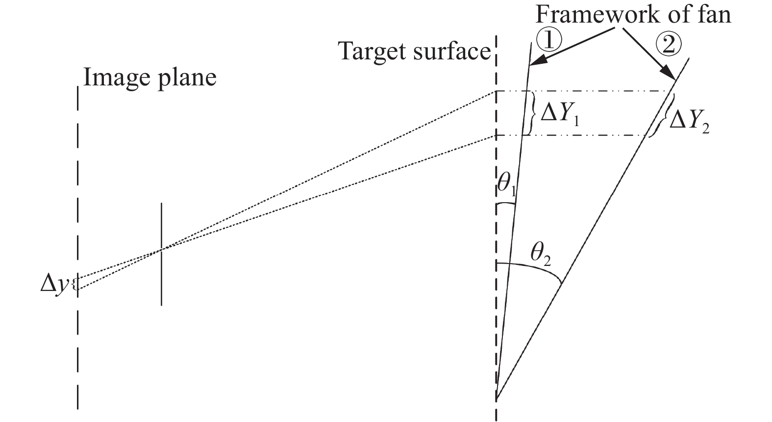
值得说明的是，目前亚像素高精度定位算法的定位精度小于0.2 pixel，因此实验中特征提取误差对参数解算精度影响较小。此外，标定扇选用$ \theta \in [ - {10^ \circ },{10^ \circ }] $的扇骨面有利于得到精确、稳定的参数解，这是由于随着$ \theta $增大，相同像素误差$ \Delta y $所引起的数据误差$ \Delta Y $增大，从而引起特征点对$ y,Y $的精度下降，致使方程组解的稳定性降低，如图6所示。此外，在参数解算过程中，标定方程的高度奇异性也可能是标定误差被放大的原因。

Figure 6.  Cause analysis of parameter solution instability

实验选用武汉汉宁轨道公司研发的钢轨测量模块中的线阵相机完成内参数标定，相机有效像元4096个，像元尺寸7 μm，镜头焦距为25 mm，相机视场明亮，光照强度均匀。图7（a）中，相机模块于导轨上匀速运动（速度为6 mm/s），距离编码器以0.2 mm/次的频率向相机发送触发采集的信号，使单个像素的分辨率小于特征圆的半径，以确保采集标靶图像中的特征圆有效。相机沿导轨运动方向采集标定扇的二维图像如图7（b）所示，其中有13列像点，每列代表单根扇骨的特征圆。运用亚像素高精度定位算法处理图像，得到各特征点的像点坐标$ y $，根据提出的标定方法完成相机标定，得到每根扇骨的参数解算结果。利用第7组数据解算的线阵相机内参数见表3。

Figure 7.  Test scene

扇骨面与靶面的旋转角$ \theta $在0°~±10°范围内时参数解算结果较稳定。图8所示为各扇骨解得的像主点坐标$ {y_0} $与焦距$ f $。其中，由第4~10根扇骨解算的相机内参数结果具有一致性，且各扇骨的$ \theta \in \left[ { - {{10}^ \circ },{{10}^ \circ }} \right] $。当扇骨面与靶面的夹角$ \left| \theta \right| > {10^ \circ } $时，参数解算结果不稳定，如第1、2、3、11、12、13扇骨，像主点和焦距的解算结果分别浮动约5 pixel和25 μm，且有随着$ \theta $增大而浮动范围增加的趋势，这与图5所得结论保持一致。

Figure 8.  The results of 13 fan bones solving $ {y_0} $ and $ f $. (a) The result of $ {y_0} $; (b) The result of $ f $

采用上述标定方法获得的稳定解可作为集成模块中线阵相机的准确内参数。为验证模型参数的正确性，将每根扇骨标定出的相机参数代入公式(4)，将标定特征点重投影到像面，原像点与重投影点之差记为重投影误差$ {\rho _c} $。第4~10根扇骨共156个特征点，用单根扇骨上12个特征点解算相机参数，将其他特征点作为检验点，计算重投影误差以验证参数的标定精度。表4给出了每根扇骨所得重投影误差的最大值、最小值、均方根误差，图9统计了所有特征点重投影误差$ {\rho _c} $的分布占比，其中89%特征点的重投影误差小于0.20 pixel，最大误差优于0.28 pixel，单根扇骨上特征点重投影误差的RMSE为0.086~0.129 pixel。需要说明的是，采集10次标定扇图像完成相机内参数求解与精度验证，其中重投影误差的平均RMSE为0.11 pixel，标准差为0.01 pixel，参数标定结果精度高且一致性好，相较于文献[18]（重投影精度为0.37 pixel），重投影精度提高了69.7%。

Figure 9.  The proportion of re-projection error distribution

另外，基于改进的L-M算法在不影响内参数标定精度的同时可有效提高计算效率。分别利用标准L-M算法和改进L-M算法优化第4~10根扇骨的参数初值，表5对比了两种优化方法的迭代次数和重投影误差的RMSE。相比于前者，改进的L-M算法将迭代次数减少约50%，而参数标定结果无明显差异。

线阵相机常与其他传感器以模块化的形式安置于设备内部，对于这类相机内参数的定期检校成本高，困难程度大。鉴于此，提出一种基于2.5D标定扇的线阵相机内参标定方法。一方面，2.5D标定扇兼具3D标靶的立体测量效果和2D标靶低成本、高精度的优点，特征点数量多分布规律，避免了特征易丢失的问题，且特征点与像点易配对。另一方面，所构建的线阵相机标定模型顾及了镜头畸变误差和靶面与像面间两个方向的小角度姿态，相机移动方向与标定物的位置无严格限定。实验表明，采用$ \theta $<±10°的扇骨标定相机内参为最佳，标定结果精度高且一致性好，其中89%特征点的重投影误差小于0.20 pixel，最大误差优于0.28 pixel，平均RMSE为0.112 pixel。此外，相比于标准L-M算法，改进的L-M算法在不影响参数优化精度的同时将迭代次数减少一半，同时避免方程在解的过程中出现奇异。

值得说明的是，该方法还适用于钢轨病害检测、车间质检、文物数字化等应用场景的线阵相机完成定期内参数检校，有利于传感器维持高精度测量状态，同时亦可为其他可见光、红外等线性光电探测器测量装置的内参数标定提供有益参考。然而，该标定方法也有局限性，要求线阵相机与标定靶面间应具有较小的姿态角以确保解算线性系数方程时$ {D_x} $、$ {D_y} $近似不变，才能获得准确的参数初值，否则会引起解的不稳定。