


-
在工业测量领域,被测物体经常具有特征稀疏,低纹理区域多,测量精度要求高等特点[1]。因此通常通过主动投射结构光[2]的方式,为物体表面增加编码的光信息,利用解码出的光信息作为特征实现高精度测量的目的。主动光栅测量方法主要分为单目光栅测量系统和双目光栅测量系统。单目光栅方法采用的是高度映射原理[3-4],研究方向多在解决投影仪和相机之间的标定关系 [5-6]。而双目光栅测量系统,往往将投射的光栅图案作为双目系统立体匹配的一个环节,难点集中在立体匹配的精度上。光栅图案有正弦光栅图案,散斑图案和二值编码条纹[7]等。
在光栅投影辅助双目视觉测量系统中,很多人对投射正弦光栅图案并利用相移法求解出的相位来进行立体匹配做了研究。其中姜宏志[8]等对图案进行极线校正后,以单点相位差值最小的点基元方法进行匹配,与传统二维匹配方式相比这种方法大大节约了匹配时间。为减少单点匹配的噪声,肖志涛[9]引入模板匹配的方式,一定程度上降低了噪声以及相位偏差对匹配精度的影响,并利用求解二维曲面最小值的方式找到匹配点。戴鲜强[10]则将条纹投影和散斑投影结合在一起,减少了所需投射图案的数目,从而加快了测量速度。上述方法是基于极线校正[11]的双目光栅投影的测量方法,在视场情况下测量效果很好。在小视场下,双目系统受到视场和环境限制夹角过大,无法保证在双相机主点坐标一致情况下进行极线校正。因而针对微小型被测物,单目的测量方法较为常见。陈超等[12]将体视显微镜,相机和投影仪相组合,利用单目光栅测量的原理实现三维重建,丁迅等[13]则研究了利用多幅图像融合的方式进行三维重构,从而获得微小物体的三维形貌,均达到了很好的重建效果。
文中提出了极线辅助的级次约束方法用于双目光栅投影测量系统中,可以在小视场下实现快速立体匹配。在立体匹配阶段,可以先通过双目系统的极线约束方程得到一维的匹配区域,再利用正弦光栅条纹展开得到的条纹级次进一步缩小待匹配区域。匹配点搜索时只在与符合约束条件匹配区域进行搜索,减少了搜索区域,并利用带权值模板匹配的方式保证了测量精度。
-
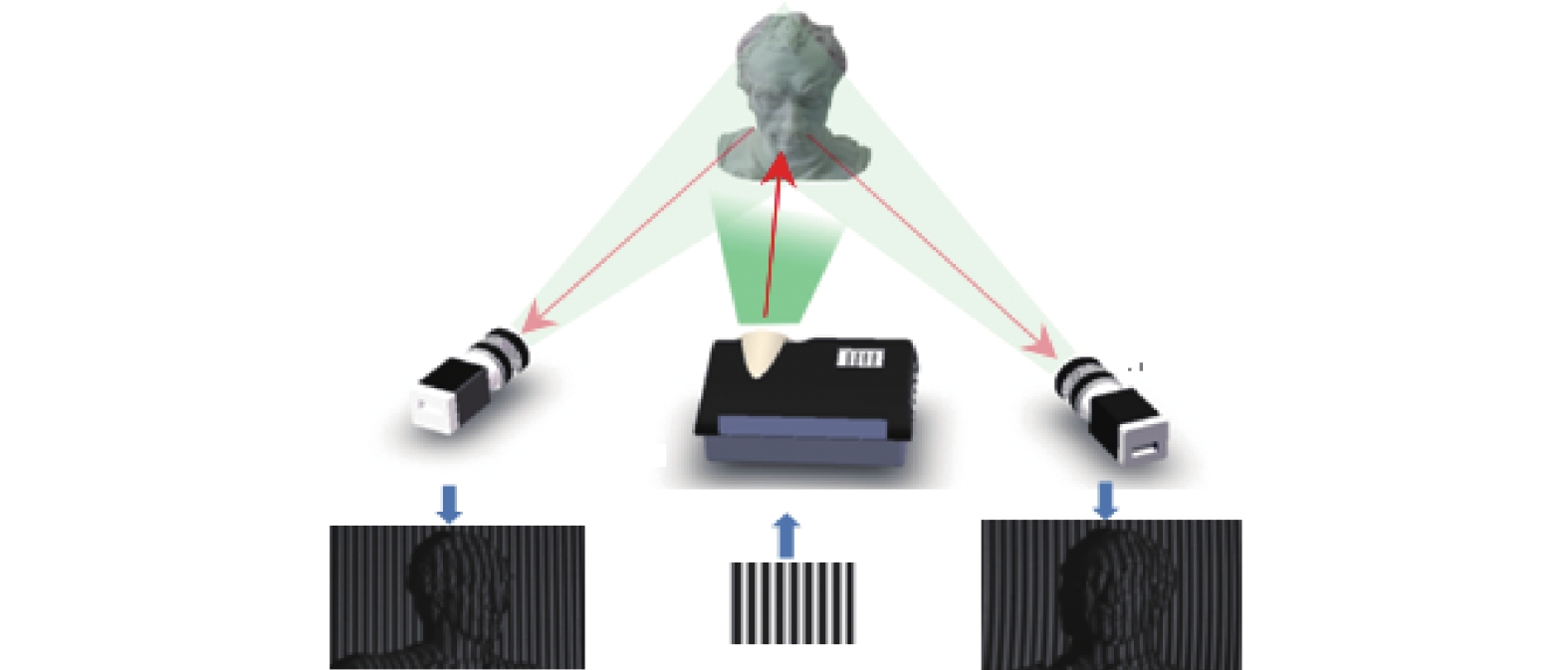
光栅辅助的双目立体视觉的测量原理如图1所示,利用DLP(Digital Light Procession)投影仪读取设定好频率的正弦光栅条纹图像,依次投射到被测物体表面,由左右相机分别采集视场范围内对应的变形光栅图像,通过双目标定,利用光栅投射的相位信息进行立体匹配得到左右图像上的对应匹配点,再通过最小二乘法得到被测物的三维坐标。

图 1 测量系统示意图
Figure 1. Diagram of measurement system
目前针对光栅投影测量系统的相位计算方法有多种,实验采用四步相移法[10],使用四步相移投射的四幅图像的相移量分别为
${I_1}$ 、${I_2}$ 、${I_3}$ ,${I_4}$ ,可得知对应像素点的包裹相位为:$$\varphi (x,y) = \arctan \left(\frac{{{I_2} - {I_4}}}{{{I_1} - {I_3}}}\right)$$ (1) 得到被测物的包裹相位的范围在(−π,π)中,需要通过三频相位展开运算得到条纹级次从而得到绝对相位:
$$\phi (x,y) = \varphi (x,y) + 2{m_0}\text{π} $$ (2) 式中:
${m_0}$ 为包裹相位所对应的条纹级次。空间中一点
$P$ 在左右相机的图像中的对应点${P_l}$ 和${P_r}$ 利用立体匹配算法被确定后,通过相机标定可以分别得到左右相机的投影矩阵${M_l}$ 和${M_r}$ 。${Z_{cl}}$ 、${Z_{cl}}$ 分别为$P$ 点在左右相机坐标系中的$Z$ 方向的坐标,根据双目相机成像模型有:$$\begin{array}{l} {Z_{cl}}{p_l} = {M_l}P \\ {Z_{cr}}{p_r} = {M_r}P \end{array} $$ (3) 求解上述方程组,从而可得到
$P$ 点的世界坐标。 -
根据透视成像原理,在双目立体系统存在极线几何关系。如图2所示,
${I_l}$ 和${I_r}$ 分别为左右相机的采集图像,点$P$ 是被测物体上一点,${P_l}$ 和${P_r}$ 分别为点$P$ 在左右两幅图像上的投影点坐标,存在对应关系为:$$p_r^{\rm{T}}F{p_l} = 0$$ (4) 式中:
$F$ 为基础矩阵,根据极线约束原理可知,左图像的一点的对应匹配点,一定位于右图像对应的极线上。反之亦然。
图 2 极线几何模型
Figure 2. Polar constraint model
在立体匹配过程中应以对应极线上的点为主要搜索点。由于极线不水平,极线会经过两个像素点中间,匹配点未必会完全的落在对应极线上,因此设置一个阈值
$\delta $ ,即:$$\frac{{\left| {p_r^{\rm{T}}F{p_l}} \right|}}{{\left| {F{p_l}} \right|}} < \delta $$ (5) 当不等式成立时,认为该点处于待匹配区域内。由此可得带匹配区域点集
${S_1}$ 。这里阈值设为0.5。 -
条纹级次的判定主要借助于投影仪向被测物投射的多组光栅条纹图像,利用三频外差法计算出的绝对相位的过程会为不同位置光栅条纹标记不同的序号。并且每个像素点计算的绝对相位值只和该点在多幅投射图像上获取到的相位值有关,而与其他像素点的相位值无关。在计算相位展开过程中,条纹频率依次选择为
${f_1} = n$ 、${f_2} = n - 1$ 、${f_3} = n - \sqrt n $ 。$n$ 可选合适的整数,下文中实验的$n = 49$ 。利用
${f_{13}} = {f_1} - {f_3} = n$ 、${f_{23}} = {f_1} - {f_2} = \sqrt n - 1$ 从而所得到的${\lambda _{13}}$ 和${\lambda _{23}}$ 两组不同波长条纹图。对于图像上的某一像素点,假设其展开相位值分别为${\phi _{13}}$ 、${\phi _{23}}$ ,$d$ 为所取相位点到0相位点横坐标距离,$m$ 为条纹级次,$\lambda $ 为条纹波长,$e$ 表示折叠相位值与$2\pi $ 的比值,范围为(0,1)。则${\phi _{13}} = 2{\text{π}} d/{\lambda _{13}}$ ,${\phi _{23}} = 2{\text{π}} d/{\lambda _{23}}$ 。二者做差后的相位值为${\phi _{123}} = 2{\text{π}} d{\lambda _{123}}$ ,${\lambda _{123}} = {\lambda _{13}}{\lambda _{23}}/({\lambda _{13}} - {\lambda _{23}})$ 。可以得到等式:$$d = ({m_{13}} + {e_{13}}){\lambda _{13}} = ({m_{123}} + {e_{123}}){\lambda _{123}}$$ (6) 根据前面选择的频率可知
${\lambda _{123}} > d$ ,则${m_{123}}$ =0,上述等式可化简为:$$ ({m_{13}} + {e_{13}}){\lambda _{13}} = {e_{123}}{\lambda _{123}} $$ (7) 因此可得到条纹级次:
$$ {m_0} = Int \left[\frac{{{\lambda _{123}}}}{{{\lambda _{13}}}}{e_{123}} - {e_{13}}\right] $$ (8) 将每一个像素点的条纹级次
${m_0}$ 保存下来,作为在立体匹配时的判断条件之一。如图3所示,为投影条纹光栅时所记录的条纹级次理想示意图。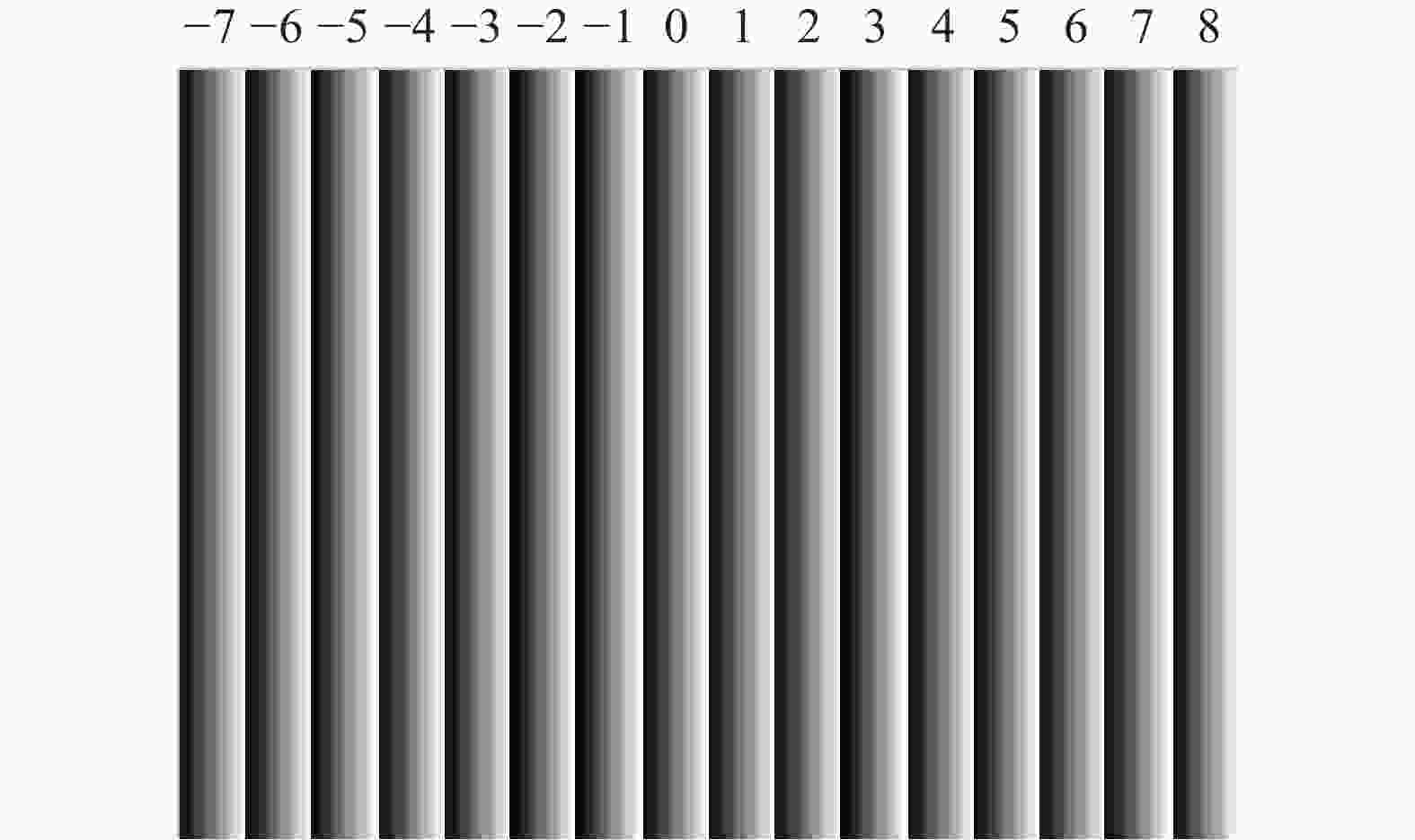
图 3 条纹解相级次图
Figure 3. Fringe phase unwrapping order graph
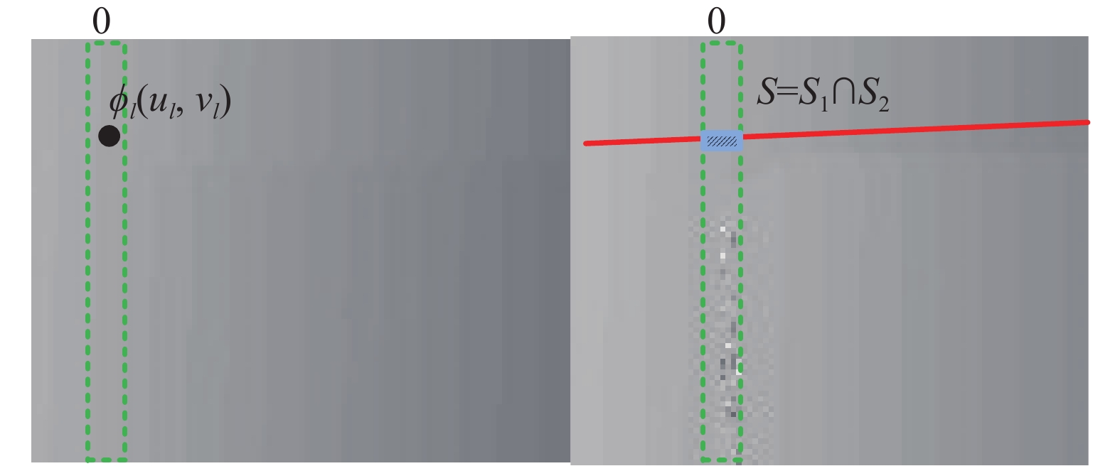
记录条纹级次后,面对左相位图
$I$ 上的一点标准相位点${\phi _l}({u_l},{v_l})$ ,其所对应的右图极线为$ax + by + $ c = 0,右相机采集到的相位图对应的待匹配区域点集$S$ 数学表达式为:$$\left\{ {\begin{aligned} & {\left\{ {S = {S_1} \cap {S_2}} \right\}} \\ & {\left\{ {{S_1}|({u_r},{v_r}) \in {S_1},|a{u_r} + b{v_r} + c| < 0.5} \right\}} \\ & {\{ {S_2}|{m_r}({S_1}) = {m_l}(({u_l},{v_l}))\} } \end{aligned}} \right.$$ (9) 如图4左侧图片为截取的一部分左相机展开相位图,选取一点
${\phi _l}({u_l},{v_l})$ ,右侧图片为对应的右相机展开相位图,其中绿色虚线框内点集为${S_2}$ ,红色粗实线覆盖区域为${S_1}$ ,两者相交的区域为待匹配点集$S$ 。
图 4 立体匹配区域示意图
Figure 4. Schematic diagram of to stereo matching area
-
在实际操作中,假设
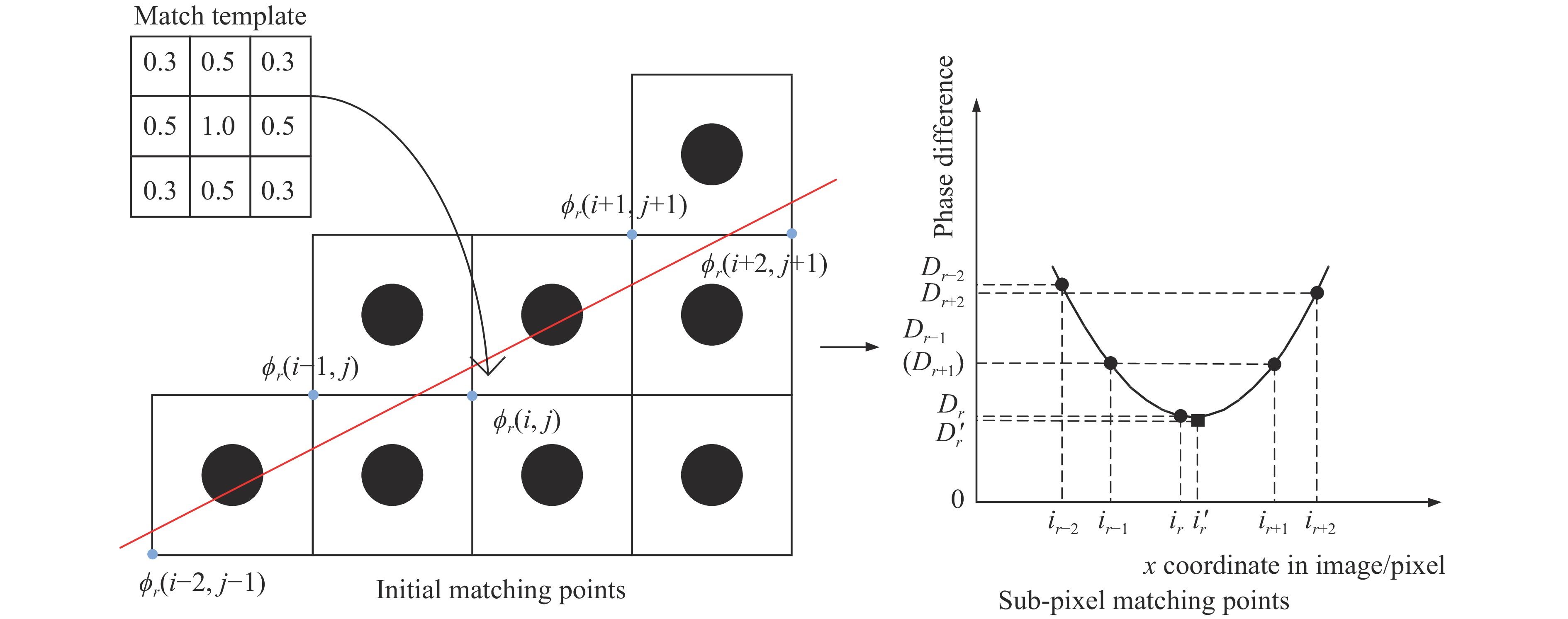
${\phi _l}(i,j)$ 为左图一点的标准相位,${\phi _{ri}}$ 为右图的某一点待匹配相位,考虑到利用单个像素点的相位值进行的匹配,容易受到噪声的影响,使用模板匹配可以减少误匹配的情况。而对于物体边缘处的相邻点易有相位突变情况,为防止边缘处模糊的情况,因此为模板不同位置赋予不同的权值。标准模板以左图的匹配点为中心,建立一个3×3窗口,按照距中心点的距离,对不同像素点上的相位值赋予不同的权值,中心点的权值为1,相邻的横纵像素点的权值为0.5,斜对角线上的权值则为0.3。如图5所示,根据该模板得到的相位总和将作为初始匹配点的判断标准。具体公式如下: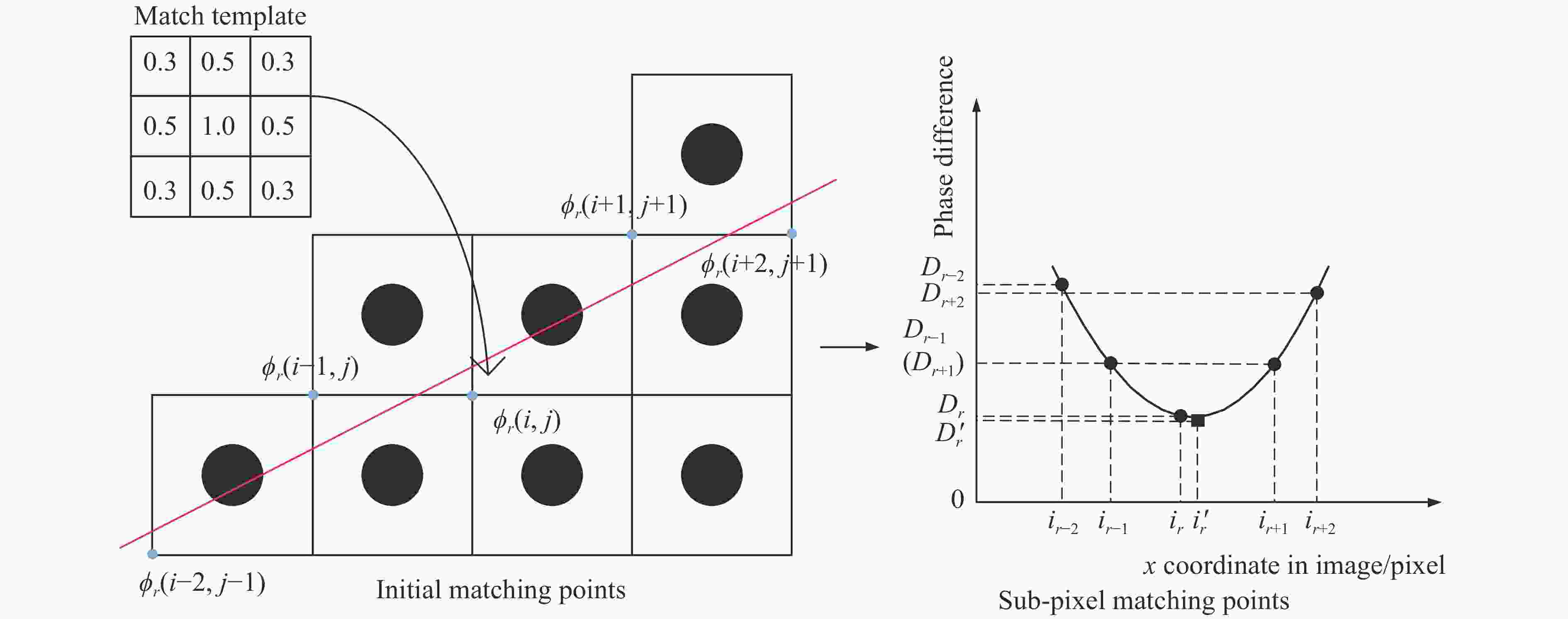
图 5 相位立体匹配过程
Figure 5. Process of stereo matching with phase
$$\begin{split} & {t_l} = \alpha \sum\limits_{y = j - 1}^{j + 1} {\sum\limits_{x = i - 1}^{i + 1} {\phi (x,y)} } \\ & {D_i} = |{t_l} - {t_i}| \end{split} $$ (10) 选取右图中与左图标准模板偏差
${D_i}$ 最小的点,即相似度最大的待匹配点确定为初始匹配点${\phi _r}(i,j)$ 。初始匹配点为像素级精度,以初始点为基准,寻找与其附近相邻的4个待匹配点的相位差绝对和${D_{r - 2}}$ ,${D_{r - 1}}$ ,${D_r}$ ,${D_{r + 1}}$ ,${D_{r + 2}}$ 代入二次曲线拟合函数$m{x^2} + nx + q = y$ ,$x$ 方向坐标值为自变量可以得到矩阵方程:$$\left[ {\begin{array}{*{20}{c}} {i_{r - 2}^2}&{{i_{r - 2}}}&1 \\ \vdots & \vdots & \vdots \\ {i_{r + 2}^2}&{{i_{r + 2}}}&1 \end{array}} \right]\left[ {\begin{array}{*{20}{c}} m \\ n \\ q \end{array}} \right] = \left[ {\begin{array}{*{20}{c}} {{D_{r - 2}}} \\ \vdots \\ {{D_{r + 2}}} \end{array}} \right]$$ (11) 利用最小二乘法求出二次曲线参数,并得到顶点的横坐标值,利用极线方程得到对应的纵坐标值。求取的亚像素级匹配坐标
$\phi _r'({i'},{j'})$ 应该满足:$$\begin{split} & {i'} = - m/2n \\ & {j'} = ( - c - a \times {i'})/b \\ \end{split} $$ (12) -
投影系统采用分辨率为1 280×720的DLP投影仪投射条纹。摄像机系统采用Basler工业相机,型号为acA2440-35 μm,分辨率为2 440×2 048,系统测量距离为400 mm,测量范围30 mm×30 mm,适用于小型被测物。相机标定过程无需标定投影仪。实验时由投影仪依次向被测物体上投射光栅条纹频率依次为49、48、42的四步相移光栅条纹图,共12幅条纹图像。并利用计算机根据文中的算法进行立体匹配,最后通过双目相机成像模型进行三维重构生成点云。
-
特征稀疏的平面不好比较单点匹配的具体情况,因此选用平面靶标作为被测对象进行实验,利用靶标上的圆心点坐标对比来进行判断匹配的准确度。将系统进行标定后,向靶标依次投射所需的条纹图,图6(a)和(b)分别为左右相机拍摄的多组光栅条纹图中的一幅,图6(c)和(d)为将对应条纹图案展开求解后所得到的绝对相位图像,也是进行立体匹配的判断标准。选取靶标图中选取49个靶标圆心在左相机图像中的坐标作为待匹配点,其对应的相位值作为待匹配相位值,分别通过传统的点基元匹配方法和与文中方法得到的右图中的匹配坐标点相位差值做比较。
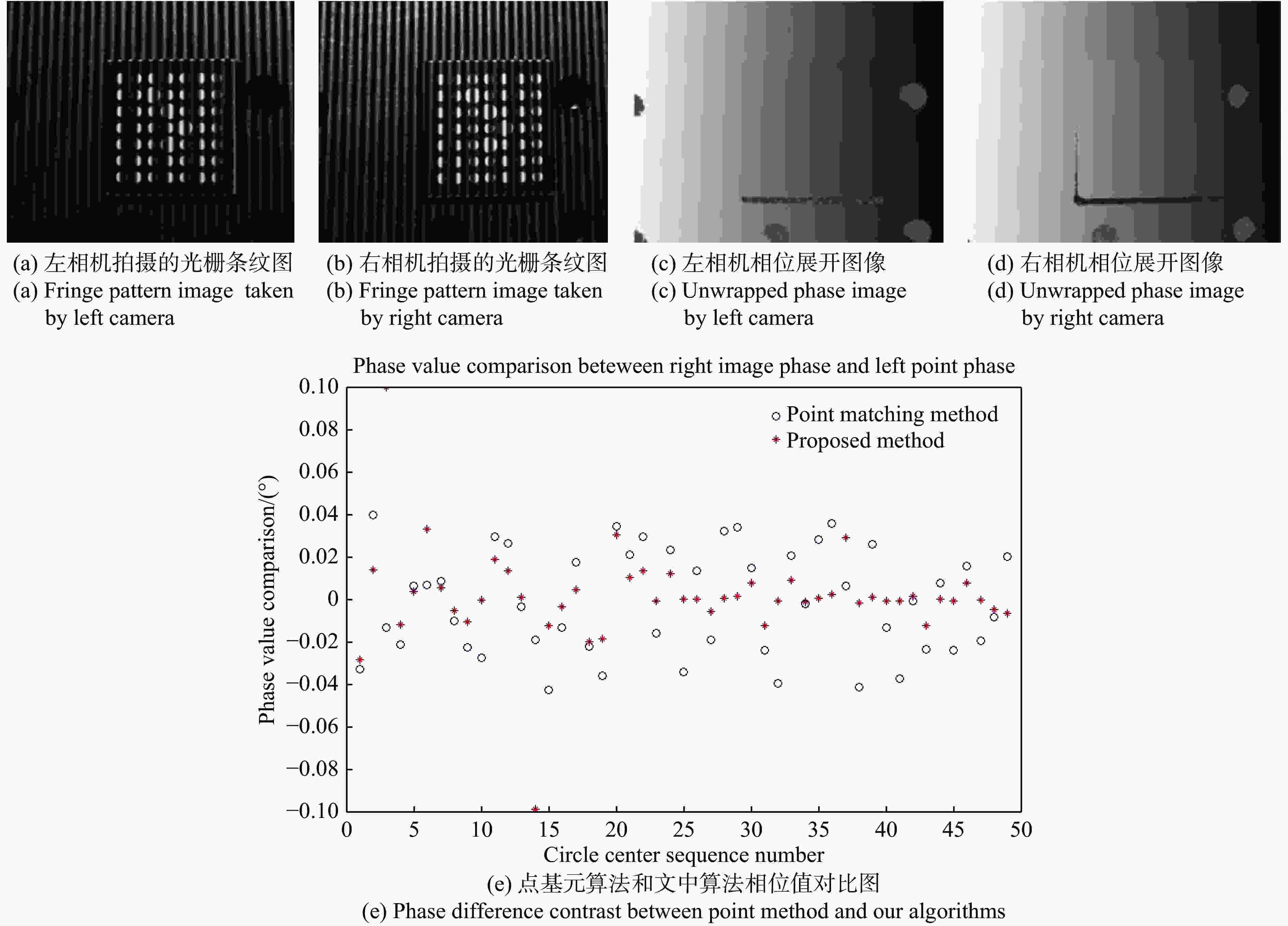
图 6 圆心点相位值分析
Figure 6. Analysis of centers phase
从图6(e)结果中可以看到,图中用圆圈表示的利用点基元的方法,得到的右图坐标点的相位值和左图待匹配点的相位值不能完全相等,范围区间在[−0.05,0.04]中波动,而使用十字表示的亚像素坐标获取方法得到的亚像素坐标点的相位值和左图待匹配点的相位值的差值明显更小,从而具有更高的匹配精度。
-
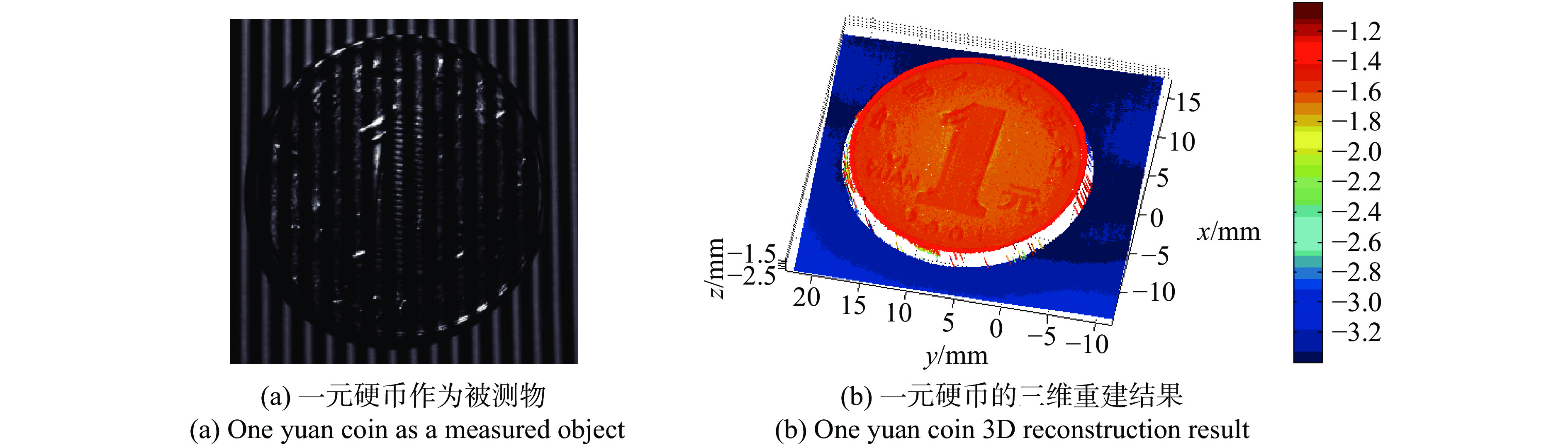
首先选取特征比较明显的一元硬币图7(a)作为被测物,也适用于本系统的视场大小。可以看到:图7(b)硬币表面的特征结果可以被很好地测量出来,可以清晰地看到硬币上的特征,三维重建效果良好。

图 7 一元硬币分析
Figure 7. Analysis of one yuan coin
另外选取图8(a)中微小半球体作为被测对象进行三维测量。同时利用只有极线约束和文中极线级次双约束两种方法进行相位匹配,可以看到图8(b)和图8(c)分别为使用文中的双约束方法和传统的极线约束实现的三维重建结果,两者均有很好的成像效果,而使用文中的方法能够减少部分相机阴影区内的杂散点。将获得的三维点云数据通过最小二乘法拟合获取半径,可以得到如表1所示的实验结果,对于半径约为5 mm的半球进行测量,测量半径平均值为
$\bar x = 5.032\;{\rm{mm}}$ ,对于半径测量重复性偏差为: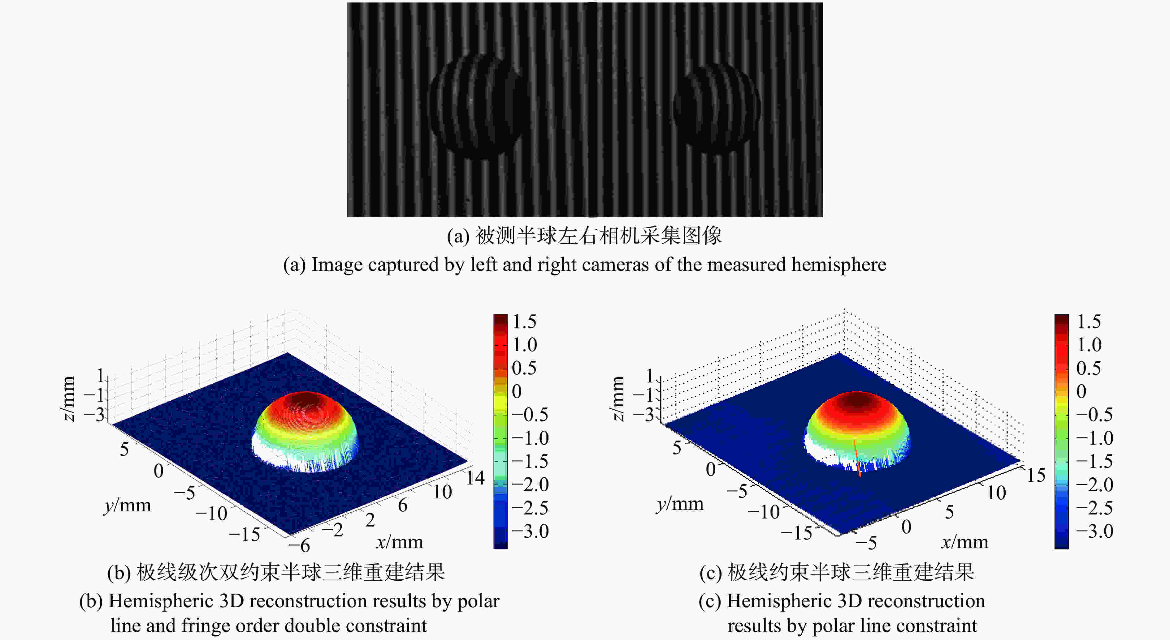
图 8 半球体作为被测物分析
Figure 8. Analysis of hemisphere as a measured object
表 1 小球半径测量实验结果
Table 1. Experiment result of hemisphere radius
Experiment serial number Radius/mm 1 5.032 2 5.028 3 5.035 4 5.030 5 5.031 6 5.029 7 5.037 8 5.030 9 5.034 10 5.035 $$s = \sqrt {\frac{1}{{N - 1}}{{\sum\limits_{i = 1}^N {({X_i} - \bar x)} }^2}} = 0.004\;{\rm{mm}}$$ (13) -
双目光栅投影系统利用投射的光栅条纹计算出的相位值,辅助双目系统的立体匹配环节,从而实现被测物体的高精度三维重建。为提高匹配环节的速度,提出了一种利用极线约束和条纹级次双约束的方法。在光栅投影辅助双目测量系统中,使用相移法求解条纹相位,借助多频外差的方式标记条纹级次,在极线约束的基础上增加了条纹级次约束来确定待匹配范围,该方法较传统的极线约束方法减少了计算量,适用于光轴汇聚式的双目系统。并采用了带权值模板匹配和亚像素精度求解的方法,保证了匹配精度。方法在小视场下实验效果很好,一元硬币作为被测物有很好的重建效果,对直径10 mm的小球,测量精度在5 μm左右,可以实现小型物体的外观和几何尺寸高精度测量。
Fringe projection measurement method based on polar line and fringe order double constraint
-
摘要: 利用结构光辅助立体视觉技术在三维测量领域可以很好地解决被测物特征稀疏的问题,从而实现对物体几何尺寸的高精度测量。提出了利用极线和条纹级次双约束的方式,通过双目相机中的极线约束原理和多频外差法得到的光栅条纹级次进行混合约束,降低了立体匹配的待匹配区域。立体匹配过程中设计了一种带权值的窗口模板,利用相位信息配合模板匹配的方式确定初始匹配点,并通过初始匹配点与附近点的相位差值利用二次曲线拟合方法实现亚像素级匹配。实验表明:该方法在较小视场测量中应用良好,对直径10 mm大小的球体可以实现快速、准确的测量。Abstract: Structured light-assisted stereo vision technology can solve the problem of the measured object with sparse characteristics, so as to realize the high precision measurement of the geometric dimension of the object.The method of using the polar line and the fringe order double constraint was proposed, which was based on the principle of polar constraint in binocular camera and fringe order in multi-frequency heterodyne. Using this method, the stereo matching area was reduced. And during the stereo matching process, a weighted image template was used, the initial matching point was determined by using the phase information and the similarity template matching method, and the sub-pixel matching was realized by the two-dimensional curve fitting method according to the spatial distance and the phase difference of the initial matching point and the polar line. Experiments show that the method is applied well in small field of view measurement, and can achieve fast and accurate measurement for spheres with a diameter of 10 mm.
-
表 1 小球半径测量实验结果
Table 1. Experiment result of hemisphere radius
Experiment serial number Radius/mm 1 5.032 2 5.028 3 5.035 4 5.030 5 5.031 6 5.029 7 5.037 8 5.030 9 5.034 10 5.035  下载: 导出CSV
-
[1] Dai Meiling, Yang Fujun, Liu Cong, et al. A dual-frequency fringe projection three-dimensional shape measurement system using a DLP 3D projector [J]. Optics Communications, 2017, 382: 294−301. doi: 10.1016/j.optcom.2016.08.004 [2] Hong Ziming, Ai Qingsong, Chen Kun. High precise 3D visual measurement of based on fiber laser [J]. Infrared and Laser Engineering, 2018, 48(8): 0803011. (in Chinese) doi: 10.3788/IRLA201847.0803011 [3] Garnica G, Padilla M, Servin M. Dual-sensitivity profilometry with defocused projection of binary fringes [J]. Applied Optics, 2017, 57: 9172−9182. [4] Wang Jianhua, Yang Yanxi. Double N-step phase-shifting profilometry using color-encoded grating projection [J]. Chinese Optics, 2019, 12(3): 616−627. (in Chinese) doi: 10.3788/co.20191203.0616 [5] Dai Shijie, Fu jinshen, Zhang Huibo, et al. Revised system calibration method of analogy binocular based on fringe projection profilmetry [J]. Infrared and Laser Engineering, 2017, 46(9): 0917003. (in Chinese) doi: 10.3788/IRLA201746.0917003 [6] Zhang Xu, Shao Shuangyun, Zhu Xiang, et al. Measurement and calibration of the intensity transform function of the optical 3D profilometry system [J]. Chinese Optics, 2018, 11(1): 123−130. (in Chinese) [7] Wang Yuemin, Zhang Zonghua, Gao Nan. Review on three-dimensional surface measurements of specular objects based on full-field fringe reflection [J]. Optics and Precision Engineering, 2018, 26(5): 1014−1027. (in Chinese) doi: 10.3788/OPE.20182605.1014 [8] Jiang Hongzhi, Zhao Huijie, Liang Xiaoyue, et al. Phase-based stereo matching using epipolar line rectification [J]. Optics and Precision Engineering, 2011, 19(10): 2520−2525. doi: 10.3788/OPE.20111910.2520 [9] Xiao Zhitao, Lu Xiaofang, Geng Lei. Sub-pixel matching method based on epipolar line rectification [J]. Infrared and Laser Engineering, 2014,44(S1): 225−230. (in Chinese) doi: 10.3969/j.issn.1007-2276.2014.z1.038 [10] Dai Xianqiang. The research pm camera calibration and matching method in binocular 3D measurement system[D]. Hangzhou: Zhejiang University, 2016. (in Chinese) [11] Loop C, Zhang Z. Computing rectifying homographies for stereo vision[C]//IEEE Computer Society Conference , 1999. [12] Chen Chao, Yu Yanqin, Huang Shujun, et al. 3D small-field imaging system [J]. Infrared and Laser Engineering, 2016, 45(8): 0824002. (in Chinese) doi: 10.3788/irla201645.0824002 [13] Ding Xun, Zhao Yuejin, Ding Yukui. Three-dimensional microscopic reconstruction of MEMS based on multi image fusion [J]. Optics and Precision Engineering, 2018, 26(5): 1275−1285. (in Chinese) doi: 10.3788/OPE.20182605.1275 -

 点击查看大图
图(8) / 表(1)
计量
- 文章访问数: 1038
- HTML全文浏览量: 495
- PDF下载量: 37
- 被引次数: 0


