


-
随着微纳米制造技术、微结构元器件加工技术的发展,机械、电子、生物等方面的研究对象已由宏观领域向微观领域转变。要实现微结构元器件的高精度加工,必须建立相应的高精度测量方法。面向微小结构的高精度三维测量已广泛应用于精密制造[1]、生物医疗[2-4]、航空航天[5-6]等领域,推动着工业制造水平的不断提高。
目前适于微小结构三维形貌的非接触式测量方法主要有:双目视觉[7]、光度立体法[8]、白光干涉法[9]、激光三角测量法[10]、结构光法[11]、聚焦恢复深度法[12-13]。其中聚焦恢复深度法(Depth from Focus,DFF)通过对单相机采集到的序列图像进行清晰度评价计算,得到清晰度最高的聚焦位置[14],进而实现三维形貌测量。DFF法避免了立体视觉中的遮挡、匹配等问题的出现,适合测量范围较小的物体,具有精度高、成本低的特点,因此得到了广泛应用。瑞典HEXAGON公司、德国Zeiss公司与德国Werth公司将单相机作为探头搭载在CMM上,实现了基于DFF方法的三维形貌测量。2013年,Mahmood M T[15]提出了非线性全变差(TV)算子作为图像清晰度评价函数实现了基于DFF的三维形貌测量。2014年,Jia H K等[16]基于DFF实现了对铝膜的三维屈曲形貌的测量。山东大学的宋江山[17]采用DFF方法对物体表面三维形貌进行测量,设计了电动显微镜测量系统,实现了微小零件的表面三维形貌的非接触测量。北京理工大学的高海波[18]提出了微纳阵列三维形貌测量方法,通过数字重聚焦算法获取焦点堆栈,最后采用DFF方法获得微纳阵列深度图从而重构表面三维形貌。长春理工大学的王志桐[13]基于DFF方法实现了微小铣削零件的表面三维形貌检测。浙江大学的武祥吉[12]设计了一套基于DFF的探针台Z向距离测量系统。
图像清晰度评价函数是基于DFF法的三维形貌测量的关键,其清晰度计算的精确度与稳定性直接决定系统测量精度。2012年,国外学者Rafael Redondo等[19]利用医学显微镜系统拍摄到的图像研究分析了Power squared、Threshold、Variance等图像清晰度评价函数的精度误差。2014年,Jia H K等[16]将图像熵评价函数引入到DFF中。2017年,褚翔[20]提出了一种改进的基于8方向的Sobel算子的清晰度评价算法,比传统的两方向的Sobel算子具备更好的抗干扰性。2018年,王志桐[13]将局域方差信息熵作为清晰度评价函数引入DFF实现三维形貌测量。
文中通过实验对常用的清晰度评价函数进行了验证,分析了存在的问题。在局域方差信息熵的基础上,提出了基于高频方差熵的图像清晰度评价函数。采用定性与定量指标对常见的清晰度评价函数与文中函数的清晰度评价曲线进行了对比。通过对文中算法所获得的清晰度评价曲线进行高斯拟合,实现系统聚焦位置的插值重构,进而实现三维轮廓的非接触测量。设计了聚焦重复性测试和高度测量实验,验证了文中方法的重复性精度。
-
DFF方法是一种基于透镜成像关系,通过聚焦分析获取高度的三维形貌恢复算法[21-22],测量方法示意图如图1所示。

图 1 基于DFF的三维形貌测量方法示意图
Figure 1. Schematic diagram of 3D profile measurement based on DFF
如图1(a)所示,硬件系统中由相机成像系统作为测量探头,计算机可通过控制高精度电动三维位移台,实现对被测物表面轮廓的扫描覆盖。
相机成像系统的作用类似于接触式测量法中的探针,但以基于图像清晰度的聚焦判定代替了传统的力接触,实现非接触的轮廓点Z轴坐标的测量,其原理如图1(b)所示。测量过程中,相机成像系统对准轮廓某个点,在Z轴方向扫描采集一组表面图像序列。对应Z轴扫描位移的不同,序列中的图像有聚焦清晰与模糊的区分。采用清晰度函数对每张图像进行清晰度数值计算,可获得离散清晰度数值与对应Z轴坐标的关系曲线。通过曲线拟合,获取曲线的清晰度最大值位置,即得到精确的聚焦位置,从而确定被测物体表面点的Z轴坐标。
在上述实现单点测量的基础上,如图1(c)所示,位移台可载着被测物沿X轴与Y轴移动,对物体表面多个点位置进行Z轴垂直扫描计算坐标,从而完成表面轮廓的形貌测量,最终形成三维点云数据(图1(d))。
-
由测量方法可知,采用DFF原理实现对被测物Z轴坐标的测量,其关键在于图像清晰度评价函数,清晰度评价值的精确和稳定决定了Z轴坐标的测量精度。
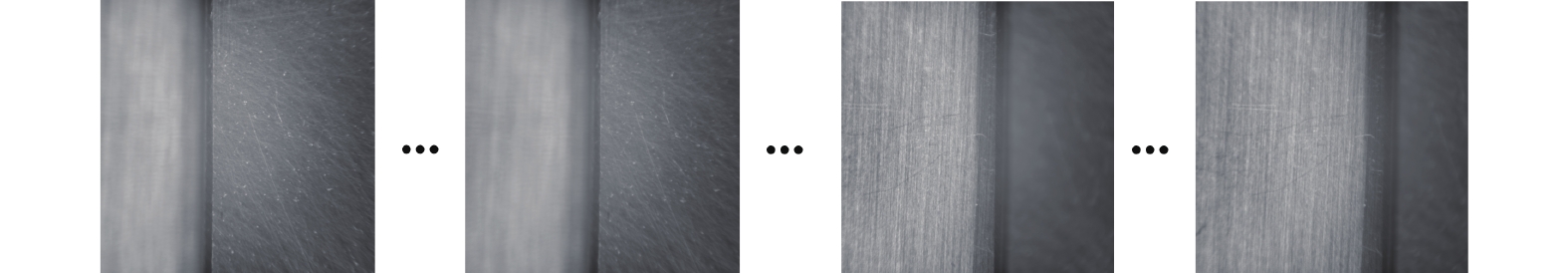
常用的清晰度评价函数有Tenengrad[23]、Brenner[24]、Laplacian[25]、Roberts[26]、Absvar[27]、信息熵(Entropy)[21]与局域方差信息熵(Local Variance Entropy, LVE)[22]。使用上述清晰度评价函数对实验采集的图像序列进行处理。采集图像序列如图2所示,相邻图像之间的实际Z轴坐标间隔为15 μm。

图 2 采集到的图像序列
Figure 2. Acquired image sequence
为了便于对比,将所有清晰度评价曲线进行了归一化处理,获取到的常用清晰度评价曲线对比图如图3所示。

图 3 常用清晰度评价函数曲线
Figure 3. Curves of the common image sharpness evaluation functions
从图3中可以看出,Absvar算法已无法判定图像序列的清晰度,信息熵算法在离焦位置清晰度数值不稳定。Tenengrad、Brenner、Laplacian、Roberts与局域方差信息熵在接近最大值点附近,其评价曲线变化趋于平缓,灵敏度降低,会引起聚焦最清晰点的位置的拟合误差,影响了后续Z轴坐标的测量精度。
-
清晰的图像比模糊的图像包含更多的信息,特别是作为图像高频分量的纹理特征。清晰的图像相比于模糊的图像,包含了更多更精细的高频分量。传统的局域方差信息熵需要计算图像中所有像素点的局域方差。然而图像中低频部分像素点的灰度都较接近,变化缓慢,计算低频部分的方差信息对整体评价算法而言影响不大。并且,局域方差信息熵对图像中存在的每一个灰度级都要进行概率计算。
在局域方差信息熵的基础上,文中提出了基于高频方差熵(High-frequency Component Variance Weighted Entropy,HCVWE)的清晰度评价函数,优化计算逻辑,只对高频部分的像素灰度进行信息熵统计计算,充分利用了图像的高频信息。HCVWE函数的定义如下:
$$ {F}_{var}=-\sum\limits_{i=1}^{n}{p}_{i}{\delta }_{({x}_{i},{y}_{i})}^{2}\ln{p}_{i} $$ (1) 式中:
$ {F}_{var} $ 为HCVWE函数计算的图像清晰度数值;n为图像高频分量的像素点个数;$ {p}_{i} $ 为第i个高频分量像素灰度级出现的概率;$ {\delta }_{({x}_{i},{y}_{i})}^{2} $ 为第i个高频分量像素的局域方差,其公式为:$$ {\delta }_{\left({x}_{i},{y}_{i}\right)}^{2}=\frac{1}{9}\sum\limits_{a=-1}^{1}\sum\limits_{b=-1}^{1}{\left[I\left({x}_{i}+a,{y}_{i}+b\right)-\mu \right]}^{2} $$ (2) 式中:
$ {\delta }_{\left({x}_{i}, {y}_{i}\right)}^{2} $ 为图像I以$ \left({x}_{i}, {y}_{i}\right) $ 为中心,3×3为邻域的局域方差;$ \mu $ 为该邻域内的灰度平均值;$ I\left({x}_{i}+a,{y}_{i}+b\right) $ 为图像$ \mathrm{在}\left({x}_{i}+a,{y}_{i}+b\right) $ 处像素点的灰度值。HCVWE使用3×3邻域对高频分量进行方差计算,重点关注高频纹理特征像素的小邻域内的统计信息,能够较好地避免图像本身灰度分布和噪声干扰,也控制了运算量。 -
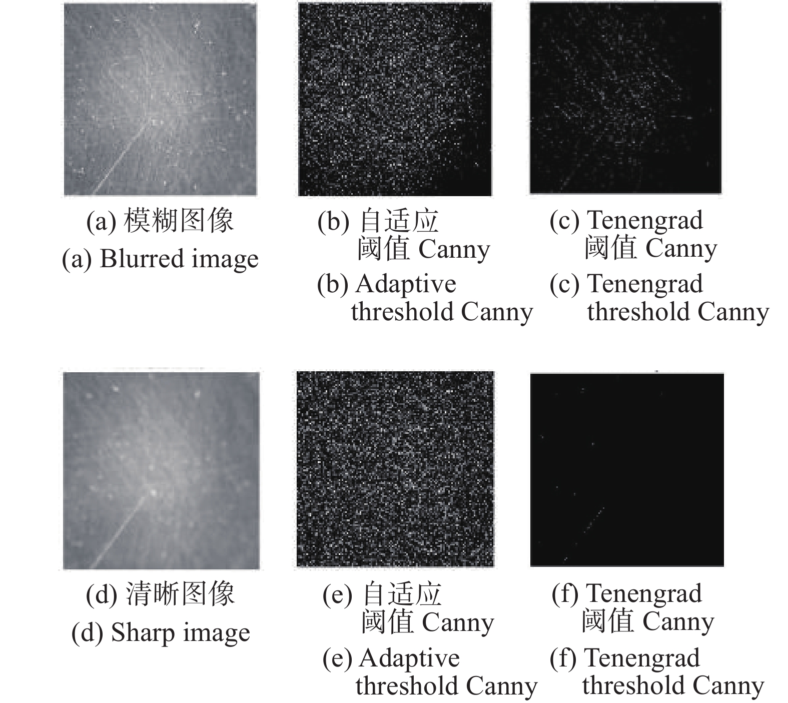
根据HCVWE的定义可知,计算流程首先要从图像中提取高频分量像素。文中采用Canny算子进行高频分量像素提取,但其阈值的选取直接影响高频分量提取的结果。文中计算序列图中每幅图像归一化后的Tenengrad梯度值用以确定序列图中对应图像Canny算子的阈值,具体计算公式如下:
$$ {k}_{m}=1-(0.8\times {\varepsilon }_{m}) $$ (3) 式中:
$ {k}_{m} $ 为适用于序列中第m张图像的Canny算子的阈值;$ {\varepsilon }_{m} $ 为序列中第m张图像的Tenengrad归一化梯度值。图4为使用自适应阈值和文中阈值方法的Canny算子进行处理的效果对比图。可以看出,自适应阈值易于受图像本身灰度分布和噪声干扰影响,对于清晰和模糊图像的提取结果均中存在较多的离散无纹理规律的像素。而文中采用Tenengrad梯度值来计算阈值,由于其与纹理特征清晰程度相关,因此在清晰图像中保留了足够的纹理特征像素点,并且抑制了噪点。

图 4 Canny算子处理结果
Figure 4. Canny operator processing result
通过Canny算子求得原图I(x, y)的高频分量图像g(x, y),从g(x, y)中获取高频分量在原图中对应像素。然后根据公式(1)对高频分量像素进行统计计算,得到清晰度评价数值。文中设计的具体计算流程如图5所示。

图 5 高频方差熵评价函数的计算流程
Figure 5. Flow chart of the calculation process of HCVWE function
-
与图3使用相同的图像序列,对HCVWE函数与常用的清晰度评价函数进行对比,清晰度评价曲线对比图如图6所示。

图 6 高频方差熵与常用清晰度评价函数曲线
Figure 6. Curves of the proposed HCVWE and common image sharpness evaluation functions
从图6可以看出,文中提出的高频方差熵评价函数在陡峭度和单峰性上都较优于其他清晰度评价算法。尤其是在最大清晰度值附近,常见的评价算法已趋于平缓,文中提出的算法在最大值处相较于其左右评价值的变化显著,可以有效判定最清晰的图像位置。
为了更客观地表达评价算法的性能,利用定量评价指标清晰度比率和灵敏度对以上清晰度评价函数进行对比分析。定义如下:
(1)清晰度比率
清晰度比率R为清晰度评价曲线中,最大值与最小值的比值,其定义如下:
$$ R = \frac{{{f_{\max }}}}{{{f_{\min }}}} $$ (4) 式中:fmax为曲线的最大值;fmin为曲线的最小值。R越大,说明通过该清晰度评价函数得到的正焦图像与离焦图像的清晰度值差异越大。
(2)灵敏度因子
灵敏度因子可以用来表征清晰度评价函数曲线最大值附近的变化程度。灵敏度因子越高,曲线最大值附近的变化越大,当灵敏度因子较小时,会影响聚焦判定的准确度。图7所示为不同评价曲线的灵敏度示意图。

图 7 灵敏度因子示意图
Figure 7. Schematic diagram of the sensitivity factor
当曲线F1,F2横坐标变化ε,其值变化分别为δ1,δ2,δ2>δ1,表明清晰度评价曲线F2的灵敏度高于F1。灵敏度因子的定义如下:
$$ {f_{{\rm{sen}}}} = \dfrac{{{f_{\max }} - f\left( {{{\textit{z}}_{\max }} + \varepsilon } \right)}}{{f\left( {{{\textit{z}}_{\max }} + \varepsilon } \right)}} $$ (5) 式中:ε = ± 1。fmax为清晰度评价曲线的最大值;f(zmax+ε)为评价曲线最大值的横坐标变化ε时,曲线的函数值。fsen越大,说明清晰度函数曲线的变化越剧烈,越有利于找到聚焦图像位置。
表1为定量评价指标对清晰度评价函数的评价结果,其中R值评价的是各函数直接计算值,而非其均一化数值。
表 1 定量评价指标
Table 1. Quantitative evaluation indexes
Functions R fsen (ε=1) fsen (ε=−1) Tenengrad 1.519 0.009 0.038 Brenner 2.338 0.012 0.017 Laplace 1.578 0.039 0.007 Roberts 1.542 0.029 0.003 LVE 4.115 0.019 0.059 HCVWE 4604.634 0.025 0.056 从表1可知,文中提出的高频方差熵函数的清晰度比率明显高出其余算法。高频方差信息熵算法的灵敏度因子总体表现较好,在保证清晰度评价曲线单峰性和无偏性的同时,有效提高了灵敏度。
-
通过运动控制系统只能实现Z轴离散位置的扫描采集,不能简单地在图像序列中寻找最清晰图像来判定聚焦位置。应通过对计算得到的清晰度评价曲线进行拟合,计算拟合曲线的峰值点来代替原始评价曲线的峰值点,该峰值点所对应的位置坐标即为聚焦点的位置[14]。文中提出的高频方差熵清晰度评价函数计算得到的曲线基本符合高斯分布的特征。因此对评价曲线采用高斯拟合方法[28-29]。高斯曲线的表达式为:
$$ y=a{\cdot {\rm e}}^{-{\left(\frac{x-b}{c}\right)}^{2}} $$ (6) 式中:a,b,c为待确定系数。对公式(6)两边取对数整理变形得到:
$$ Y=A{x}^{2}+Bx+C $$ (7) 其中:
$$ \left\{\begin{array}{c}Y=-\ln y \\ A=1/{c}^{2} \\ B=-2b/{c}^{2} \\ C={b}^{2}/{c}^{2}-{\rm ln}a\end{array}\right. $$ (8) 参数A,B,C可由最小二乘原理确定,然后计算参数a,b,c:
$$ \left\{\begin{array}{c}a={\rm e}^{\left({B}^{2}/4A-C\right) }\\ b=-B/2A \\ c=\sqrt{1/A} \end{array}\right. $$ (9) 图8为对高频方差熵清晰度评价函数曲线的高斯拟合结果,可以求得拟合曲线最大值对应的被测点Z轴坐标位置为229.125 μm。

图 8 高斯拟合结果
Figure 8. Gaussian fitting result
-
根据DFF测量方法,文中设计搭建了一套实验平台,硬件系统实物图如图9所示,其中精密位移台的型号为DZLPC20-60-3W,其三维行程均为20 mm,微步运动时重复定位精度<1 μm。利用搭建的实验平台,测试了聚焦重复性完成高度测量实验。

图 9 硬件系统实物
Figure 9. Hardware system
-
实验采用一标准量块,验证系统的聚焦判定性能,测试流程为:位移台在Z轴方向在不同的起始位置与终点位置间运动,相机对量块表面进行扫描,采集多组图像序列,经过文中提出的高频方差熵清晰度函数处理后,通过高斯拟合计算得到的聚焦点所在位置,从而验证聚焦清晰位置测量的重复性。
实验选取了8组不同起始位置与终点位置,垂直扫描步进为15 μm,每组扫描范围逐渐缩小。测试数据如表2所示。测量聚焦清晰位置的平均值为641.969 μm,标准差为2.820 μm。
表 2 聚焦重复性测试数据(单位:μm)
Table 2. Data of the focusing repeatability test data (Unit: μm)
Scanning range Focusing position 15-1350 644.520 60-1305 641.414 105-1260 644.303 150-1215 645.675 195-1170 637.527 240-1125 640.032 285-1080 642.689 330-1035 639.590 Average value 641.969 Standard deviation 2.820 -
选择标准高度台阶验证测量精度与重复性。实验采用由标准量块组成的1.5 mm高的台阶进行测试,标准高度台阶如图10所示。

图 10 标准高度台阶
Figure 10. Standard height step
对台阶表面采点扫描测量,每个采集点在X轴与Y轴的间隔距离为0.2 mm,在每个采集点上进行Z轴垂直扫描的步进为0.015 mm,X轴扫描范围为0.67~3.87 mm,Y轴扫描范围为−0.3~0.3 mm。图11为扫描台阶采集图像的过程。

图 11 扫描采集图像过程
Figure 11. Scanning and image acquisition process
采用最小二乘法对系统测量得到的三维点云进行平面拟合,标准台阶上表面的平面拟合方程为0.007x + 0.039y − z + 2.238 =0,下表面的平面拟合方程为0.003x + 0.013y − z + 0.751 = 0。实际测量点和台阶拟合效果图如图12所示。

图 12 标准台阶测量结果
Figure 12. Measurement result of the standard step
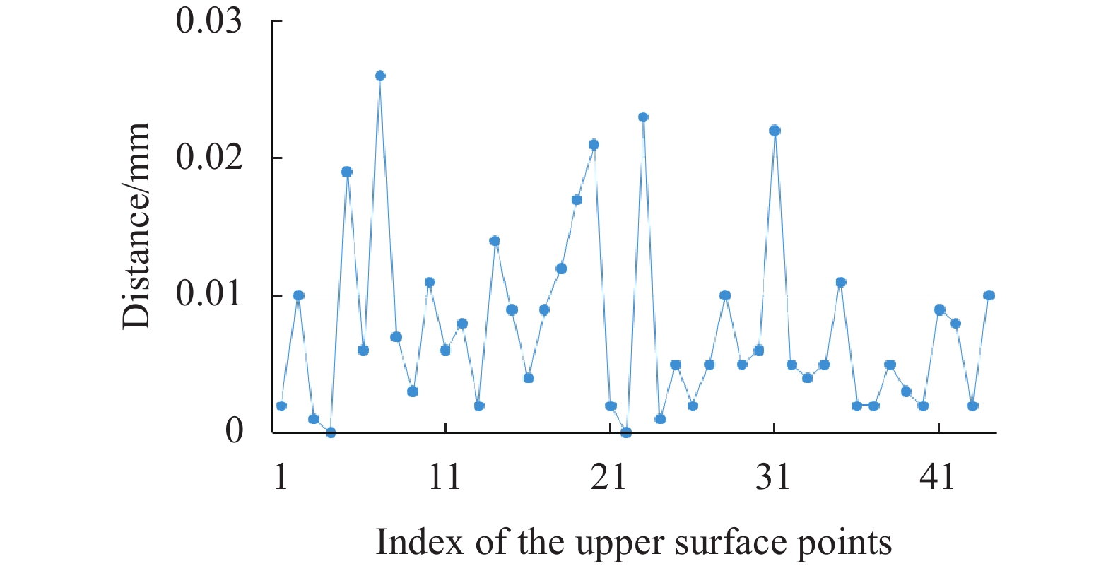
上表面的三维点到下表面平面的垂直距离数据如图13所示,上表面点到上表面平面的垂直距离数据如图14所示,下表面点到下表面平面的垂直距离数据如图15所示。

图 13 上表面点到下平面距离
Figure 13. Distance from each upper surface point to the lower plane
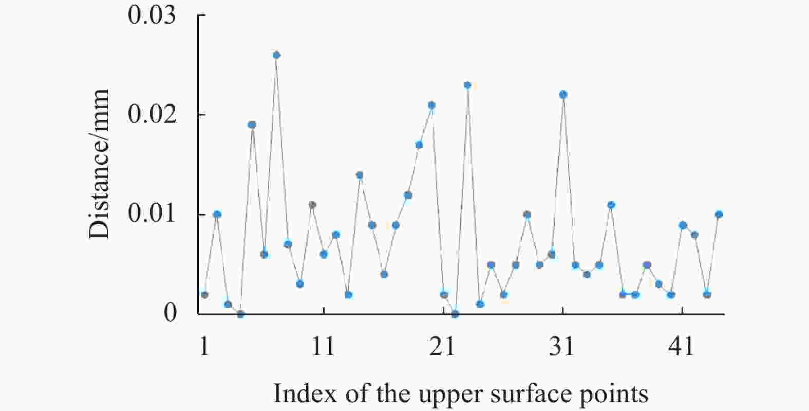
图 14 上表面点到上表面平面距离
Figure 14. Distance from each upper surface point to the upper plane

图 15 下表面点到下表面平面的垂直距离
Figure 15. Distance from each lower surface point to the lower plane
台阶上表面三维点云到下表面拟合平面的平均距离为1.499 mm,标准差为0.012 mm。上表面三维点云到上表面拟合平面的平均距离为0.008 mm,标准差为0.007 mm。下表面三维点云到下表面拟合平面的平均距离为0.007 mm,标准差为0.006 mm。
-
文中提出了基于高频方差信息熵的图像清晰度评价函数,用于基于DFF测量方法的三维测量。对常见的清晰度评价函数与文中函数进行了定性与定量指标对比。通过对文中清晰度评价函数获取的曲线进行高斯拟合,实现了系统聚焦位置的精确测量。在验证实验中,选取标准量块与1.5 mm高的标准台阶作为被测对象,进行了聚焦重复性与高度测量测试。进行8次重复性聚焦实验,测量标准差为2.82 μm;利用1.5 mm标准台阶完成了高度测量,台阶高度测量平均值为1.499 mm,标准差为0.012 mm。
3D profile measurement based on depth from focus method using high-frequency component variance weighted entropy image sharpness evaluation function
-
摘要: 图像清晰度评价函数是聚焦恢复深度法(Depth from Focus, DFF)实现三维形貌测量的核心,直接决定了深度方向的测量精度。文中提出了一种基于高频方差熵的图像清晰度评价函数,与常用函数对比了清晰度比率、灵敏度因子两个定量指标,结果表明所提函数优于常用函数。通过对所提函数获得的清晰度评价曲线进行高斯曲线拟合,实现了深度方向聚焦位置的精确计算。对文中方法开展了聚焦重复性与标准台阶高度测量测试,重复性聚焦实验的测量标准差为2.82 μm,台阶高度测量标准差为12 μm,验证了文中方法用于高精度非接触三维测量的可行性。Abstract: Image sharpness evaluation function is the core of Depth from Focus (DFF) method for 3D profile measurement. Crucially, the accuracy of depth measurement is determined by the evaluation function. An image sharpness evaluation function using high-frequency component variance weighted entropy was proposed. The quantitative indicators including the resolution ratio and the sensitivity factor were used to test the proposed function and the common functions. The comparative data showed that the proposed function could achieve better focusing performance than the other functions. The focusing position in depth direction could be precisely confirmed by implementing the Gaussian fitting to the image sharpness curve calculated through the proposed function. Focusing repeatability and standard step height measurement were tested. The standard deviation of the data of the focusing repeatability experiment was 2.82 μm. And the standard deviation of the measurement height of the standard step was 12 μm. The result verifies the feasibility of the proposed method for high precision non-contact 3D measurement.
-
图 1 基于DFF的三维形貌测量方法示意图
Figure 1. Schematic diagram of 3D profile measurement based on DFF
图 6 高频方差熵与常用清晰度评价函数曲线
Figure 6. Curves of the proposed HCVWE and common image sharpness evaluation functions
图 14 上表面点到上表面平面距离
Figure 14. Distance from each upper surface point to the upper plane
图 15 下表面点到下表面平面的垂直距离
Figure 15. Distance from each lower surface point to the lower plane
表 1 定量评价指标
Table 1. Quantitative evaluation indexes
Functions R fsen (ε=1) fsen (ε=−1) Tenengrad 1.519 0.009 0.038 Brenner 2.338 0.012 0.017 Laplace 1.578 0.039 0.007 Roberts 1.542 0.029 0.003 LVE 4.115 0.019 0.059 HCVWE 4604.634 0.025 0.056  下载: 导出CSV
表 2 聚焦重复性测试数据(单位:μm)
Table 2. Data of the focusing repeatability test data (Unit: μm)
Scanning range Focusing position 15-1350 644.520 60-1305 641.414 105-1260 644.303 150-1215 645.675 195-1170 637.527 240-1125 640.032 285-1080 642.689 330-1035 639.590 Average value 641.969 Standard deviation 2.820
下载: 导出CSV
-
[1] Farokhi Hamed, Ghayesh Mergen H. Electrically actuated MEMS resonators: Effects of fringing field and viscoelasticity [J]. Mechanical Systems and Signal Processing, 2017, 95: 345-362. doi: 10.1016/j.ymssp.2017.03.018 [2] Simanca E, Morris D, Zhao L, et al. Measuring progressive soft tissue change with nasoalveolar molding using a three-dimensional system [J]. Journal of Craniofacial Surgery, 2011, 22(5): 1622-1625. doi: 10.1097/SCS.0b013e31822e8ca0 [3] Yamamoto S, Miyachi H, Fujii H, et al. Intuitive facial imaging method for evaluation of postoperative swelling: A combination of 3-dimensional computed tomography and laser surface scanning in orthognathic surgery [J]. Journal of Oral and Maxillofacial Surgery, 2016, 2506: e1-e10. [4] Wu C, Bradley D, Garrido P, et al. Model-based teeth reconstruction [J]. ACM Transactions on Graphics, 2016, 35(6): 1-13. [5] Zhou Peng, Zhao Fuling, Lv Qichao, et al. A surface evaluation method of carbon fiber reinforced plastic based on multifractal spectrum [J]. Journal of Dalian University of Technology, 2011, 51(4): 535-539. (in Chinese) [6] Park D C, Kim S S, Kim B C, et al. Wear characteristics of carbon-phenolic woven composites mixed with nano-particles [J]. Composite Structures, 2006, 74(1): 89-98. doi: 10.1016/j.compstruct.2005.03.010 [7] Cao Zhile, Yan Zhonghong, Wang Hong. Summary of binocular stereo vision matching technology [J]. Journal of Chongqing University of Technology (Natural Science), 2015, 29(2): 70-75. (in Chinese) [8] Zuo Chao, Zhang Xiaolei, Hu Yan, et al. Has 3D finally come of age?-An introduction to 3D structured-light sensor [J]. Infrared and Laser Engineering, 2020, 49(3): 0303001. (in Chinese) doi: 10.3788/IRLA202049.0303001 [9] Kumar U P, Wang Haifeng, Mohan N K, et al. White light interferometry for surface profiling with a colour CCD [J]. Optics & Lasers in Engineering, 2012, 50(8): 1084-1088. doi: 10.1016/j.optlaseng.2012.02.002 [10] Sun Xingwei, Yu Xinyu, Dong Zhixu, et al. High accuracy measurement model of laser triangulation method [J]. Infrared and Laser Engineering, 2018, 47(9): 0906008. (in Chinese) doi: 10.3788/IRLA201847.0906008 [11] Bai Jingxiang, Qu Xinghua, Feng Wei, et al. Separation method of overlapping phase-shift gratings in three-dimensional measurement of double projection structured light [J]. Acta Optica Sinica, 2018, 38(11): 150-156. (in Chinese) [12] Wu Xiangji. Z-distance measuring system of probe station based on automatic focusing technology[D]. Hangzhou: Zhejiang University, 2017. (in Chinese) [13] Wang Zhitong. Study on 3D image detection techniques for surface topography of micro-milling parts[D]. Changchun: Changchun University of Science and Technology, 2018. (in Chinese) [14] Nayar S K, Nakagawa Y. Shape from focus [J]. IEEE Transactions on Pattern Analysis and Machine Intelligence, 1994, 16(8): 824-831. doi: 10.1109/34.308479 [15] Mahmood M T. Shape from focus by total variation [C]//IEEE IVMSP, 2013, 6611940: 1-4. [16] Jia H K, Wang S B, Li L A, et al. Application of optical 3D measurement on thin film buckling to estimate interfacial toughness [J]. Optics & Lasers in Engineering, 2014, 54(1): 263-268. [17] Song Jiangshan. Study on depth from focus technology[D]. Jinan: Shandong University, 2009. (in Chinese) [18] Hu Yao, Gao Haibo, Yuan Shizhu, et al. 3D profile measurement of micro-structured array with light field microscope [C]//Proc SPIE, 2015, 9795: 979523. [19] Redondo R, Bueno G, Valdiviezo J C, et al. Autofocus evaluation for brightfield microscopy pathology [J]. Journal of Biomedical Optics, 2012, 17(3): 036008. [20] Chu Xiang, Zhu Lianqing, Lou Xiaoping, et al. Dynamic auto focus algorithm based on improved sobel operator [J]. Journal of Applied Optics, 2017, 38(2): 237-242. (in Chinese) [21] Lin J. Divergence measures based on the Shannon entropy [J]. IEEE Transactions on Information Theory, 1991, 37(1): 145-51. doi: 10.1109/18.61115 [22] Li Chengchao, Yu Zhanjiang, Li Yiquan, et al. Sharpness evaluation of microscopic detection image for micro parts [J]. Semiconductor Optoelectronics, 2020, 41(1): 103-107. (in Chinese) [23] Pan Xuejuan, Zhu Youpan, Pan Chao, et al. Simulation analysis of auto focusing sharpness evaluation function for images based on gradient operator [J]. Infrared Technology, 2016, 38(11): 960-968. (in Chinese) [24] Li Qi, Feng Huajun, Xu Zhihai, et al. Digital image sharpness evaluation function [J]. Acta Photonica Sinica, 2002, 31(6): 736-738. (in Chinese) [25] Wang Na, Zhou Quan. 3D reconstruction of micro objects under optical microscope [J]. Opto-Electronic Engineering, 2010, 37(11): 84-90. (in Chinese) [26] Gao Zan, Jiang Wei, Zhu Kongfeng, et al. Auto-focusing algorithm based on roberts gradient [J]. Infrared and Laser Engineering, 2006, 35(1): 117-121. (in Chinese) doi: 10.3969/j.issn.1007-2276.2006.01.026 [27] Li Xue, Jiang Minshan. A comparison of sharpness functions based on microscopes [J]. Optical Instruments, 2018, 40(1): 28-38. (in Chinese) [28] Zhang Xiaobo, Fan Fuming, Cheng Lianglun. Improvement for fast auto-focus system using laser triangulation [J]. Infrared and Laser Engineering, 2012, 41(7): 1784-1791. (in Chinese) doi: 10.3969/j.issn.1007-2276.2012.07.019 [29] Tang Chong, Hui Huihui. Gaussian curve fitting solution based on Matlab [J]. Computer & Digital Engineering, 2013, 41(8): 1262-1263+1297. (in Chinese) -

 点击查看大图

计量
- 文章访问数: 399
- HTML全文浏览量: 184
- PDF下载量: 42
- 被引次数: 0


