碳纤维复合材料因质量轻、强度高、耐高温，被广泛应用于航空航天领域^[1]。随着使用量的增加，越来越多的复合材料构件采用自动纤维铺放技术生产(Automated Fiber Placement，AFP)。受铺放路径、压辊压力、预热温度等影响，复合材料表面会出现缺丝、间隙、重叠、褶皱、扭转、架桥、气泡、异物等缺陷^[2]。起初采用人工方式对缺陷进行检测，但检测耗时过长(约占生产时间32%^[3])。为缩短检测时间，各铺放团队将检测系统前置，开发出复合材料在线检测系统。

按检测传感器种类划分，可分为可见光检测与热红外检测。基于可见光图像的检测系统，如文立伟等^[4]将可见光相机与UMAC结合，可实现间隙、重叠类缺陷的检测与铺放头的闭环控制。魏天舒等^[5]使用图像分割算法提取缺陷边缘，并对缺陷进行分类。由于复合材料可见光图像的对比度过低，因此仅对与背景亮度差异较大的缺陷，检测效果较好。

基于热红外图像的检测系统是利用复合材料铺放过程中需要热激励源对其加热，不同种类的缺陷由于热传导方式、热传导率的不同，在红外图像中与正常铺放表面差异明显。最早由波音公司将热红外相机集成进AFP系统中^[6]。Denkena等^[7-8]根据红外图像中温度的极值点，设置阈值分割缺陷所在区域，可以检测出扭转、间隙、重叠、架桥、异物类缺陷。Chen等^[9]设计了一种可用于智能决策、参数优化与质量追溯的基于红外视觉的复合材料缺陷检测系统。王璇等^[10]设计了一种基于红外图像的复合材料表面检测网络AFP-CenterNet，可以实现在无GPU加速的情况下以4.2 fps的检测速度对间隙、缺丝、扭转、气泡、起皱、异物进行检测。Gregory等^[11]采用信息重建与视频分析，对缺陷定位与评估。Juarez等^[12]采用机器学习的方法，利用热红外相机对重叠、间隙、褶皱、脱粘、扭转类缺陷进行检测，并发现借助红外热成像可以对铺放层间粘性减弱缺陷进行检测。最近，NASA^[13]提出了一种基于红外热成像的复合材料缺陷检测系统ISTIS，借助红外热图像，实时检测复合材料铺放过程中产生的重叠与间隙缺陷。并将该系统部署在NASA Langley的AFP系统中进行在线测试，可以检测出实际尺寸在0.762 mm内的缺陷。上述研究证明，热传导方式、热传导率突变的缺陷在基于红外图像的检测系统中检测效果更好。

在上述研究的基础上，康硕等^[14]首先建立一种红外与可见光联立的复合材料检测系统。分别将红外图像与可见光图像输入两个CSP-DarkNet网络中，对得到的特征图采用改进的特征金字塔网络结构进行多尺度预测。结果较单光谱检测mAP提高6.3%，证实采用红外与可见光联立的方式可以进一步提升复合材料的检测效果。

从检测结果来看，复合材料检测系统由单一的目标检测向可获取缺陷轮廓的实例分割网络发展。传统的目标检测网络仅能获取缺陷的尺寸位置信息，无法获取缺陷轮廓、面积等细化信息。为了更好辅助现场人员识别缺陷、保证产品的质量溯源，Sacco等^[15-16]提出了一种基于深度学习的缺陷分割算法。在线获取可见光图像，对缺丝、间隙、重叠、扭转、褶皱类缺陷进行检测，并对图像进行语义分割，记录缺陷轮廓。将网络嵌入AFP铺层表面缺陷检测系统ACSIS中，检测准确率可达75%以上。

由于复合材料缺丝、扭转类缺陷长宽比在12~4之间，属于狭长形缺陷。而常规卷积核具有空间尺度的局限性，很难从图像全局的角度进行综合判断，因此对上述缺陷的检测是复合材料检测的难点。为了解决卷积核只能聚合局部空间信息的劣势，目前计算机领域主流方法是将Transformer变换引入CNN网络中^[17]，增强网络对非局部空间信息的整合。在目标检测(DETR^[18]、Deformable-DETR^[19])、图像分割(SETR^[20])任务中取得亮眼的成效。将引入Transformer的网络进一步细分，可以分为Pure-Transformer架构(如ViT^[21])，和CNN+Transformer架构(如BoTNet^[22])。Pure-Transformer架构需要在大型训练集中进行预训练，再运用在特定数据集中微调模型，否则难以收敛；同时缺乏对于偏置的归纳能力。而CNN+Transformer架构是将Transformer核心机制（自注意力机制）变形为模块，插入CNN架构中，其兼具CNN平移不变性的优点以及Transformer获取全局信息的能力。

文中设计了一种基于Transformer的复合材料多源图像实时实例分割网络Trans-Yolact(Transformer Yolact)。选择检测效果最优的红外与可见光联立检测方式，在检测网络中并联图像分割模块，实时对复合材料缺陷进行检测、分类、分割。针对复合材料缺陷特点，空间域上引入Transformer变换，通道域上改进主干网络信息提取方式，进一步优化网络。第1节介绍了复合材料图像数据集的拍摄方式，红外与可见光图像的矫正、配准方式，并分析复合材料缺陷特点。第2节根据缺陷特点与基准Yolact网络特点，有针对性的提出改进方法，并详细阐述Transformer增强网络获取图像全局信息的数学原理。第3节从网络收敛的稳定性、检测的准确性对网络进行验证。并在此基础上，对网络进行剪枝优化，部署在复合材料实时检测系统中，进行在线验证。

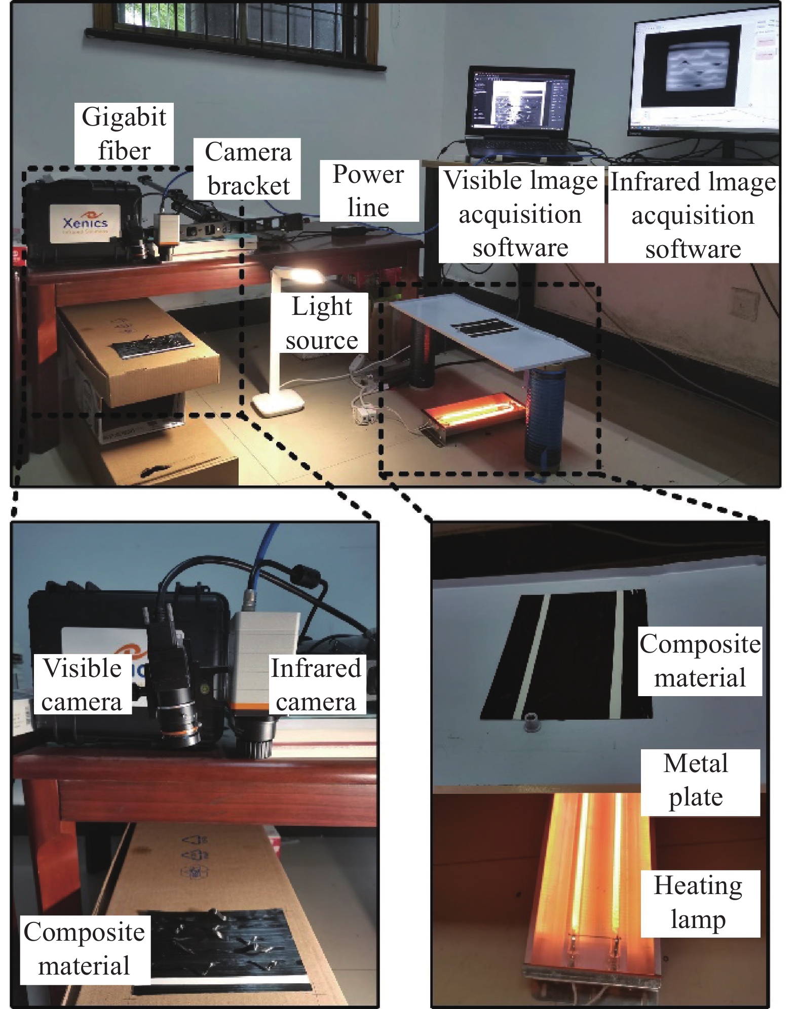
文中主要讨论复合材料常见的缺丝、扭转、异物、褶皱、架桥、气泡6类缺陷。在生产过程中采集缺陷，效率较低，无法满足深度学习所需的数据量。为此我们搭建复合材料图像采集平台。如图1所示，采集平台由红外相机、可见光相机、加热灯、可见光光源等组成。所用面阵红外相机型号为Xenics Gobi+640，相机分辨率为640×480，镜头焦距为10 mm，可以采集8~14 μm波段的热红外图像。面阵可见光相机型号为海康MV-CA013-21 UM，相机分辨率为1280×1024，镜头为MVL-HF0828 M-6 MPE，镜头焦距为8 mm。

图  1  复合材料缺陷图像采集平台

Figure 1.  Acquisition platform of composite material defect image

实际铺放过程中，需要用加热灯对基板均匀加热至90 ℃，而后使用压辊将待铺放的复合材料压实在基板表面。在拍摄图像时模拟上述铺放过程，使用加热灯加热金属薄板并保持其温度在80~110 ℃，将复合材料铺放在金属薄板上，模拟热量由基板传导至复合材料中。铺放若干秒后，将复合材料移动至拍摄区域，使用红外和可见光相机采集缺陷图像。

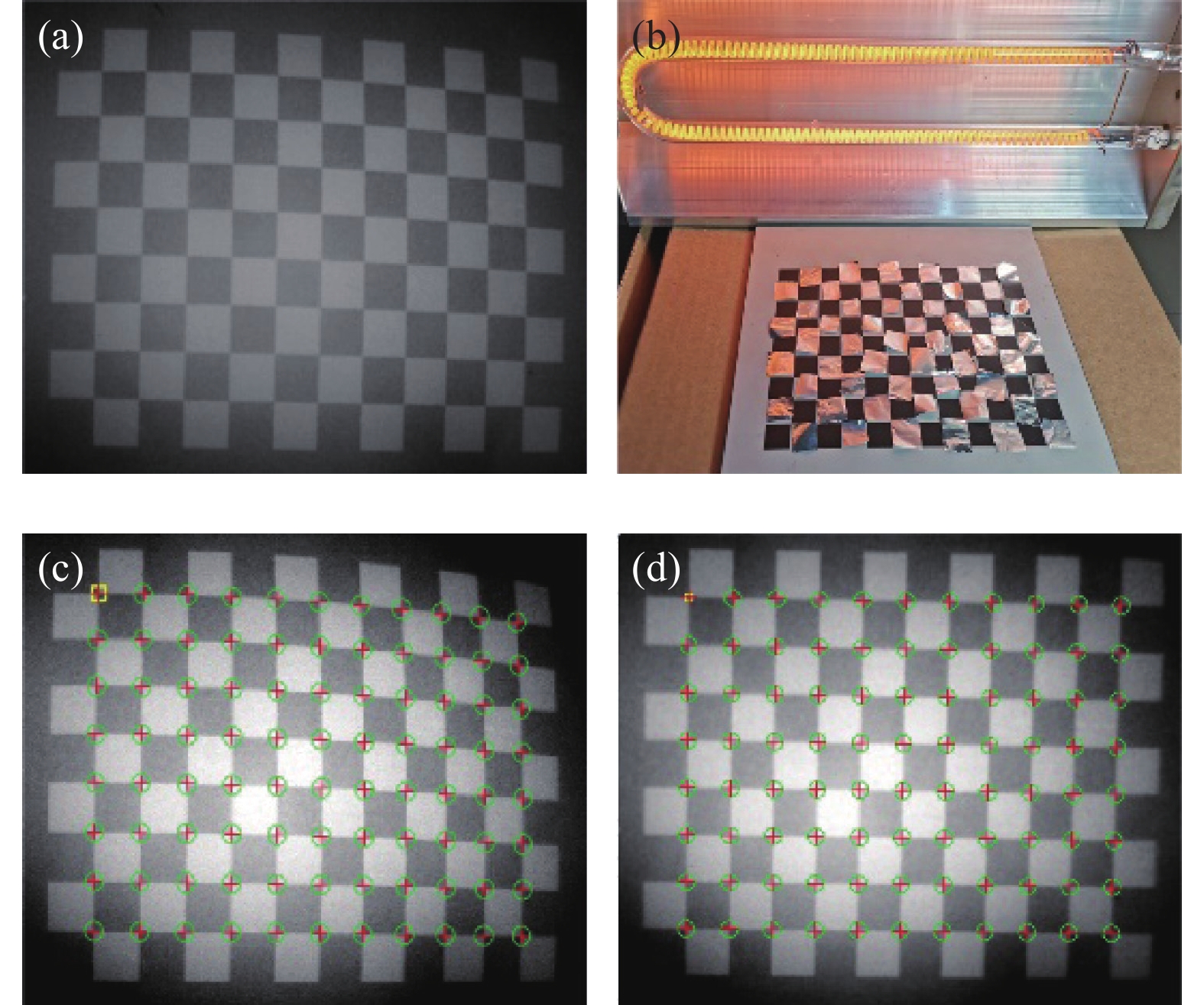
因拍摄距离较近，红外图像的畸变十分严重。需要对红外相机进行标定，而后利用相机内参对红外图像畸变进行矫正。文中采用氧化铝标定板，在红外相机标定过程中，黑色块吸收红外热辐射更多，在红外图像中更亮；白色块对光反射能力更强，在红外图像中更暗。但由于标定板经哑光处理，白色块仍能吸收一定的红外热辐射。采用张氏标定法^[23]处理时，存在部分特征点无法准确识别，见图2(a)。将锡箔贴在白色块上见图2(b)，增加白色块对红外辐射的反射能力，得到标定图像可以准确识别全部特征点见图2(c)。通过特征点求解红外相机内参数，对红外图像进行畸变矫正，结果见图2(d)。

图  2  (a)原红外图像；(b)增强标定板反射；(c) 红外图像畸变矫正前；(d)红外图像畸变矫正后

Figure 2.  (a) Infrared image; (b) Enhance the reflection of the calibration plate; (c) Infrared image before distortion correction; (d) Infrared image after distortion correction

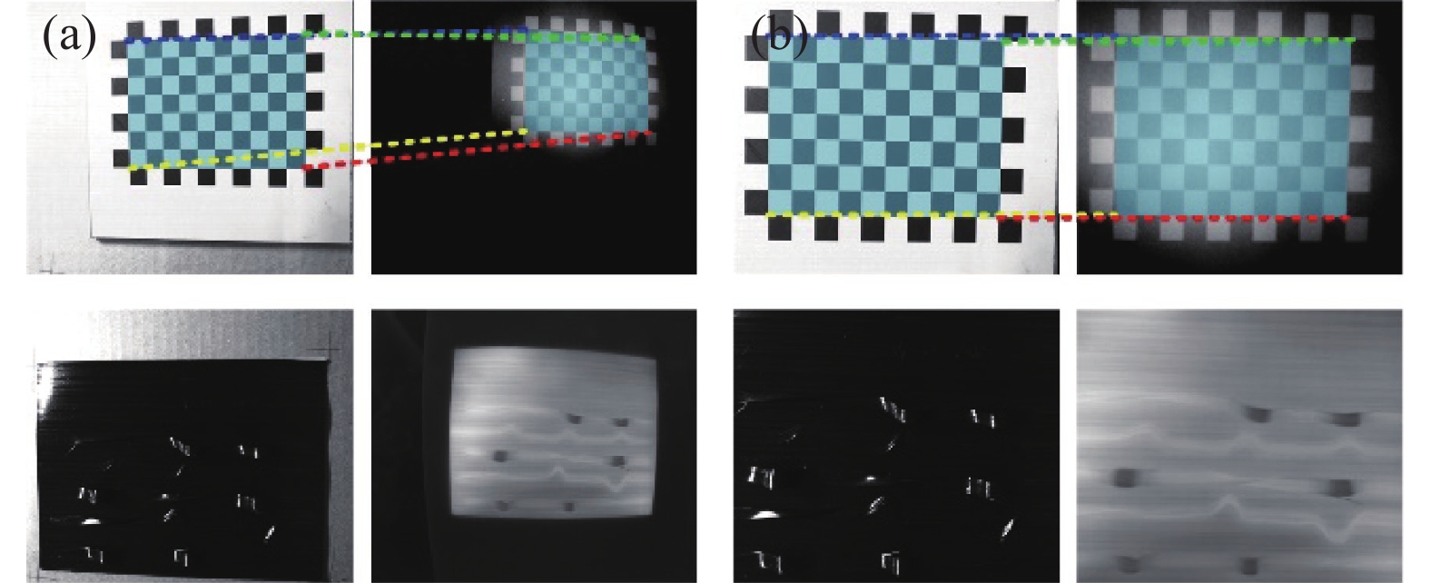
矫正红外图像后，由于红外相机与可见光相机光心与光轴不同，导致图像存在差异，见图3(a)，需要对图像进行配准。因图像采集过程中，红外相机与可见光相机的相对位置保持不变，且标定板所在平面与复合材料铺放平面重合，所以借助图像的仿形变换可以实现图像的快速配准。借助标定板的四个角点，红外图像中坐标为$\left\{\left({x}_{IR}^{1},{y}_{IR}^{1}\right),\cdots ,\left({x}_{IR}^{4},{y}_{IR}^{4}\right)\right\}$，可见光图像中坐标为$\left\{\left({x}_{VI}^{1},{y}_{VI}^{1}\right),\cdots ,\left({x}_{VI}^{4},{y}_{VI}^{4}\right)\right\}$，通过公式（1）可以求出仿形变换矩阵${M}$。后续所有可见光图像均通过上述仿形变换矩阵配准至红外相机视角，见图3(b)。

式中：$ ({x}_{VI},{y}_{VI}) $为平面一点在可见光图像中的坐标；$ ({x}_{IR},{y}_{IR}) $为该点在红外图像中的坐标；$ {d}_{x} $、$ {d}_{y} $为图像间在x、y轴上的平移量；$ {\gamma }^{n} $为表征图像间旋转、放缩、斜切的参数。

图  3  (a) 仿形变换前；(b) 仿形变换后

Figure 3.  (a) Before transformation; (b) After transformation

按上述方法采集到共计1634个不同的复合材料缺陷图像，其中包含扭转(428)、褶皱(350)、架桥(359)、气泡(273)、缺丝(110)、异物(114)。可见光图像配准、红外图像矫正后如图4(a)、(b)，对缺陷采用coco数据集格式进行实例分割标注见图4(c)。

图  4  (a) 可见光图像；(b) 红外图像；(c) 缺陷标签

Figure 4.  (a) Visible image; (b) Infrared image; (c) Defect label

观察红外图像和可见光图像，总结复合材料缺陷特点如下：（1） 大多数缺陷在红外或可见光图像中均可识别，但少数缺陷则只能在特定图像中进行识别。如扭转和部分缺丝仅能在红外图像中识别；某些异物由于导热良好，其表面温度与铺放表面温度一致，仅能在可见光图像中识别。（2） 综合红外与可见光图像信息，可以更有效的对某些种缺陷进行识别。例如架桥类、气泡，复合材料脱离铺放表面，迎光面上会出现反光带，在可见光图像中更亮，同时因脱离基板温度更低，在红外图像中更暗。（3）缺丝与扭转类缺陷，属于狭长形缺陷；部分异物类缺陷，属于尺寸较大形缺陷。上述超出CNN卷积核感受野范围，常规的卷积难以获取全部信息。

实例分割网络通常是串联目标检测网络与语义分割网络，即首先对图像进行目标检测，再对预测框内图像进行分割。典型的如Mask-RCNN，这种方法检测时间较长(>100 ms)、检测帧数较低(<8 fps)，无法应用于实时检测领域。Yolact^[24]网络则首先采用并联设计，在目标检测网络中并行接入掩膜分支如图5所示，将实例分割任务分解为两个并行的子分支，目标检测分支与掩膜分支。从而缩短检测时间(<60 ms)、提升检测帧数(>30 fps)，满足实时检测的要求。

图  5  Yolact网络结构

Figure 5.  Network structure of Yolact

在复合材料在线检测中，铺放设备的最大铺放速度约为0.8~1.2 m/s。而单张图像所能检测的范围约为80~100 mm。计算可知网络需要至少15 fps的检测帧数，才能保证不漏检缺陷。因此，文中选择目标检测分支与语义分割分支并联的Yolact网络为基础框架，保证网络检测帧数满足要求。

文中在Yolact网络框架基础上，从以下3个方面改进，使之能够更好的检测复合材料缺陷。（1）针对复合材料缺丝、扭转等狭长形缺陷，常规的卷积核具有空间尺度的局限性，在主干网络深层引入CNN+Transformer模块，增加主干网络对非局部信息的整合能力；（2） 针对复合材料架桥、气泡、异物等缺陷，需要综合红外与可见光图像信息进行判断。改进主干网络浅层，将其分为可见光通道、红外通道、混合通道，并在混合通道中引入基于通道域的注意力机制(SE模块)，增强混合通道对红外与可见光图像综合判断能力；（3） 针对Yolact网络采用图像金字塔类型的FPN结构，不同深度特征层间无法进行语义沟通，将其改进为基于Transformer的FPN结构，增强不同深度特征层、不同空间域间信息的沟通。

Trans-Yolact网络结构如图6所示，由主干网络、FPN网络、目标检测分支与掩膜分支组成。将红外图像$ \mathrm{I}\mathrm{R} $与可见光图像$ \mathrm{V}\mathrm{I} $变换至$ {\mathbb{R}}^{1\times 550\times 550} $输入主干网络图6(b)中，主干网络由浅至深提取出一系列特征图像(C1、C2、C3、C4、C5)。之后将C3、C4、C5特征层输入基于Transformer的FPN结构中，见图6(c)，生成预测图像(P3、P4、P5、P6、P7)。将提取的全部预测图像输入目标检测分支，见图6(d)，目标检测分支在预测物体种类、候选框偏移量的基础上，增加对掩膜权重值${W}_{\rm{{Mask}}}\left\{\alpha ,\beta ,\gamma ,\cdots ,\delta \right\}\in {\mathbb{R}}^{32}$的预测。对得到的候选框进行非极大值抑制筛选（Non-maximum suppression, NMS），得到目标检测输出。掩膜分支与目标检测分支并行，见图6(e)，将主干网络的浅层特征图像C3输入其中。掩膜分支通过全卷积网络(Fully convolutional network, FCN)生成32张分辨率高的非局部原型掩膜$\mathrm{M}\mathrm{a}\mathrm{s}\mathrm{k}\left\{{\mathrm{M}\mathrm{a}\mathrm{s}\mathrm{k}}^{1},{\mathrm{M}\mathrm{a}\mathrm{s}\mathrm{k}}^{2},\cdots , {\mathrm{M}\mathrm{a}\mathrm{s}\mathrm{k}}^{32}\right\}\in {\mathbb{R}}^{32\times 138\times 138}$，将原型掩膜与目标检测分支得到的掩膜权重值进行线性组合（见公式（2）），得到图像的语义分割输出$ \mathrm{S}\mathrm{e}\mathrm{g}\in {\mathbb{R}}^{1\times 138\times 138} $。最终将分割图像放缩至源图像大小，并与目标检测结果融合，得到对某一个缺陷的实例分割输出。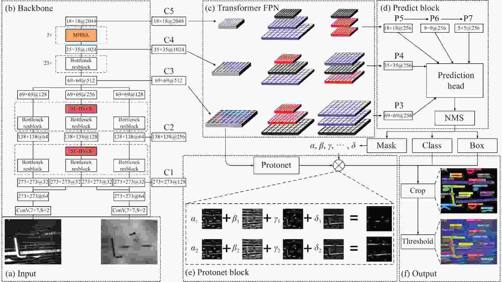

图  6  Trans-Yolact网络结构

Figure 6.  Network structure of Trans-Yolact

Trans-Yolact主干网络采用基于CNN+ Transformer架构的BoTNet网络，增加主干网络从高维特征图像中获取全局语义信息的能力。核心是将主干网络最深层C5块组，替换为多头自注意力机制模块(Multi-Head Self-Attention, MHSA)，如图7所示。

图  7  MHSA结构

Figure 7.  Multi-Head Self-Attention structure

MHSA模块可视为输入矩阵$ {X}\in {\mathbb{R}}^{d\times W\times H} $到输出矩阵${{Z}}\in {\mathbb{R}}^{d\times W\times H}$的映射。其中d是矩阵$ {X} $的通道数，W是图像的宽度，H是图像的高度。

对输入矩阵$ {X} $进行卷积核为$ {W}^{Q},{W}^{K},{W}^{V} $的1×1的卷积。将卷积结果宽度维度W与高度维度H上信息整合为一维向量，得到查询矩阵、键矩阵和值矩阵$ Q,K,V $。

接下来，对$ {Q} $、${K} $、${V} $进行编码，分为内容编码(Content)与位置编码(Position)。内容编码建立起键矩阵$ {K} $和查询矩阵$ {Q} $的内容关系矩阵$ \text{Content} $，维度为$ {{R}}^{n\times \left(W\cdot H\right)\times \left(W\cdot H\right)} $，其中n代表多头注意力机制的头数。借助内容编码，图像中某点会与图像全局的任意一点产生关联，因此可以增加网络从图像全局获取信息的能力。位置编码引入宽度维度权重参数$ {R}_{w}\in {\mathbb{R}}^{d\times W\times 1} $与高度维度权重参数$ {R}_{h}\in {\mathbb{R}}^{d\times 1\times H} $，扩展相加后得到空间域键矩阵${R}\in {\mathbb{R}}^{d\times W\times H}$。位置编码建立起空间域键矩阵${R}$与查询矩阵${Q}$的位置关系矩阵$ \text{Position} $，可以增强Transformer保留矩阵空间域信息的能力。

将上文得到的$ \text{Content} $与$ \text{Position} $加和，并进行归一化操作，得到自注意力矩阵$ {A}{t}{t} $。将值矩阵$ V $与自注意力矩阵$ {A}{t}{t} $进行矩阵相乘，可以将值矩阵$ V $映射为输出矩阵，完成Transformer的解码操作。

复合材料缺陷有时需要综合红外与可见光图像中的信息进行判断，因此对主干网络通道域进行改进。在主干网络C1模块中分别对红外与可见光图像$ \mathrm{I}\mathrm{R},\mathrm{V}\mathrm{I}\in {\mathbb{R}}^{1\times 550\times 550} $进行卷积，得到$ {\mathbb{R}}^{64\times 273\times 273} $。从卷积结果中分别提取$ {\mathbb{R}}^{32\times 273\times 273} $矩阵拼接在一起形成新矩阵$ {\mathrm{M}\mathrm{i}\mathrm{x}}_{\mathrm{C}1} $。采用先卷积、后沿通道方向拼接的方法，可以利用卷积核的感受野消除部分红外与可见光图像配准误差。C1模块输出为${\mathrm{I}\mathrm{R}}_{\mathrm{C}1},{\mathrm{V}\mathrm{I}}_{\mathrm{C}1}\in {\mathbb{R}}^{32\times 273\times 273},{\mathrm{M}\mathrm{i}\mathrm{x}}_{\mathrm{C}1}\in {\mathbb{R}}^{64\times 273\times 273}$，划分为红外通道、可见光通道、融合通道。三种通道分别侧重主干网络从红外、可见光、综合红外与可见光中获取信息。在C2、C3模块中，红外通道与可见光通道采用普通的ResNet模块。而融合通道需要综合红外图像和可见光图像中的信息，因此在ResNet模块后采用基于通道域的注意力机制(SE模块^[25])增强整合不同通道间内容的能力，如图6(b)所示。同时考虑SE模块串联接入网络中，会增加网络正向传播时间、降低网络的检测帧数。而主干网络的浅层更接近红外与可见光源图像，浅层的特征图能更好的反应红外与可见光的差异性。因此融合通道仅在主干网络的浅层(C2、C3块组)添加SE模块。最终将$ {\mathrm{I}\mathrm{R}}_{\mathrm{C}3},{\mathrm{V}\mathrm{I}}_{\mathrm{C}3}\in {\mathbb{R}}^{128\times 69\times 69},{\mathrm{M}\mathrm{i}\mathrm{x}}_{\mathrm{C}3}\in {\mathbb{R}}^{256\times 69\times 69} $拼接在一起，作为C3模块输出$ {\mathbb{R}}^{512\times 69\times 69} $送入C4模块中。

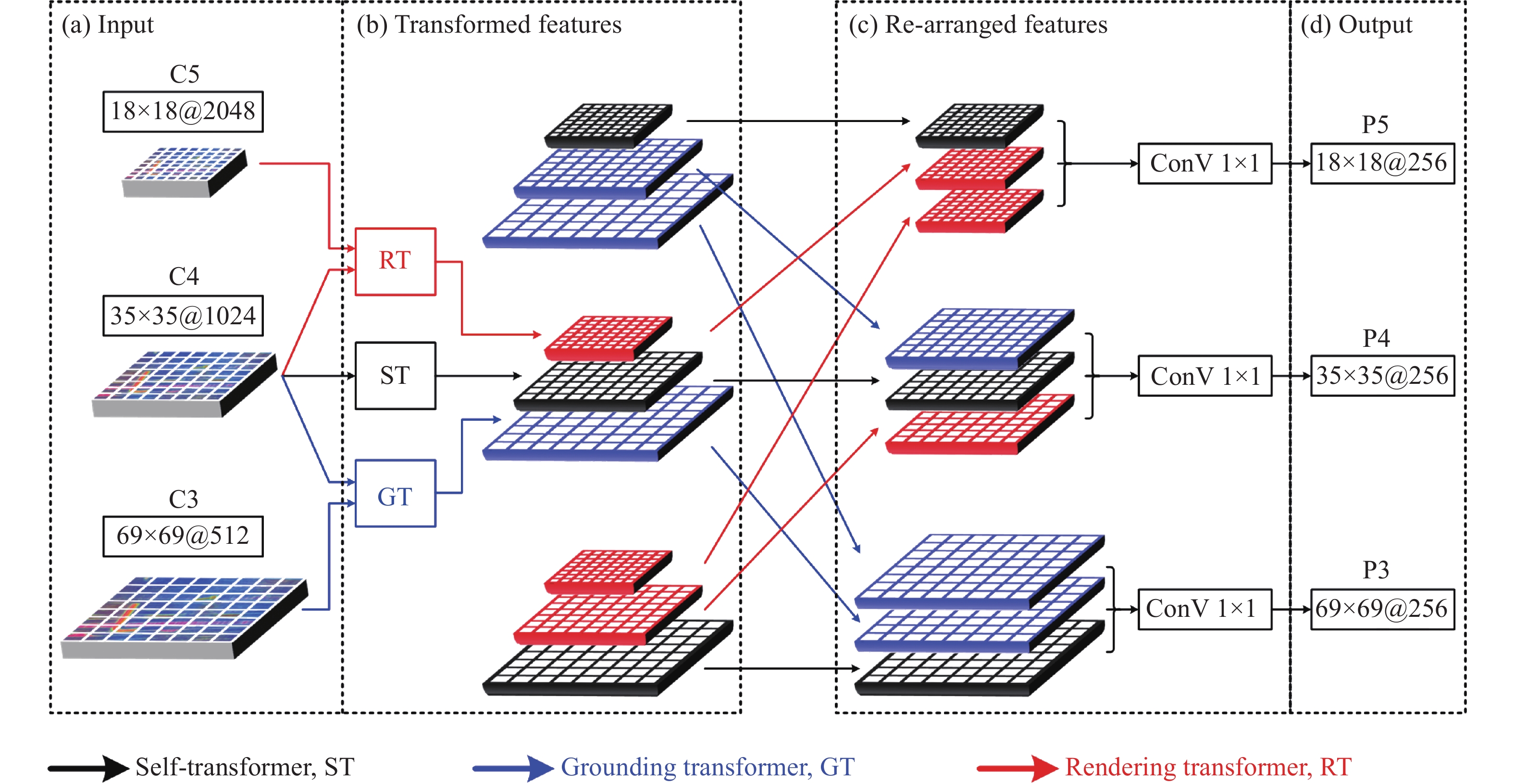
Yolact网络采用图像金字塔类型的FPN结构，这种结构的预测分支直接对特征图像进行预测，虽可缩短FPN传播时间，但缺少不同深度特征图像间的语义沟通。将Transformer变换引入FPN结构中，如图8所示，不仅可以增强不同深度特征层间的沟通，同时也可以提高特征图像空间域的信息交流^[26]。具体的，基于Transformer的FPN结构可分为基于自身的Transformer变换(Self-Transformer, ST)、深层特征增强浅层特征的Transformer变换(Grounding Transformer, GT)、浅层特征增强深层特征的Transformer变换(Rendering Transformer, RT)。

图  8  引入Transformer的FPN结构

Figure 8.  FPN structure based on Transformer

ST变换如图9(a)所示，其是对输入矩阵${X}\in {\mathbb{R}}^{d\times W\times H}$自身的Transformer变换，由于其变换方式与MHSA模块类似，在此不多赘述。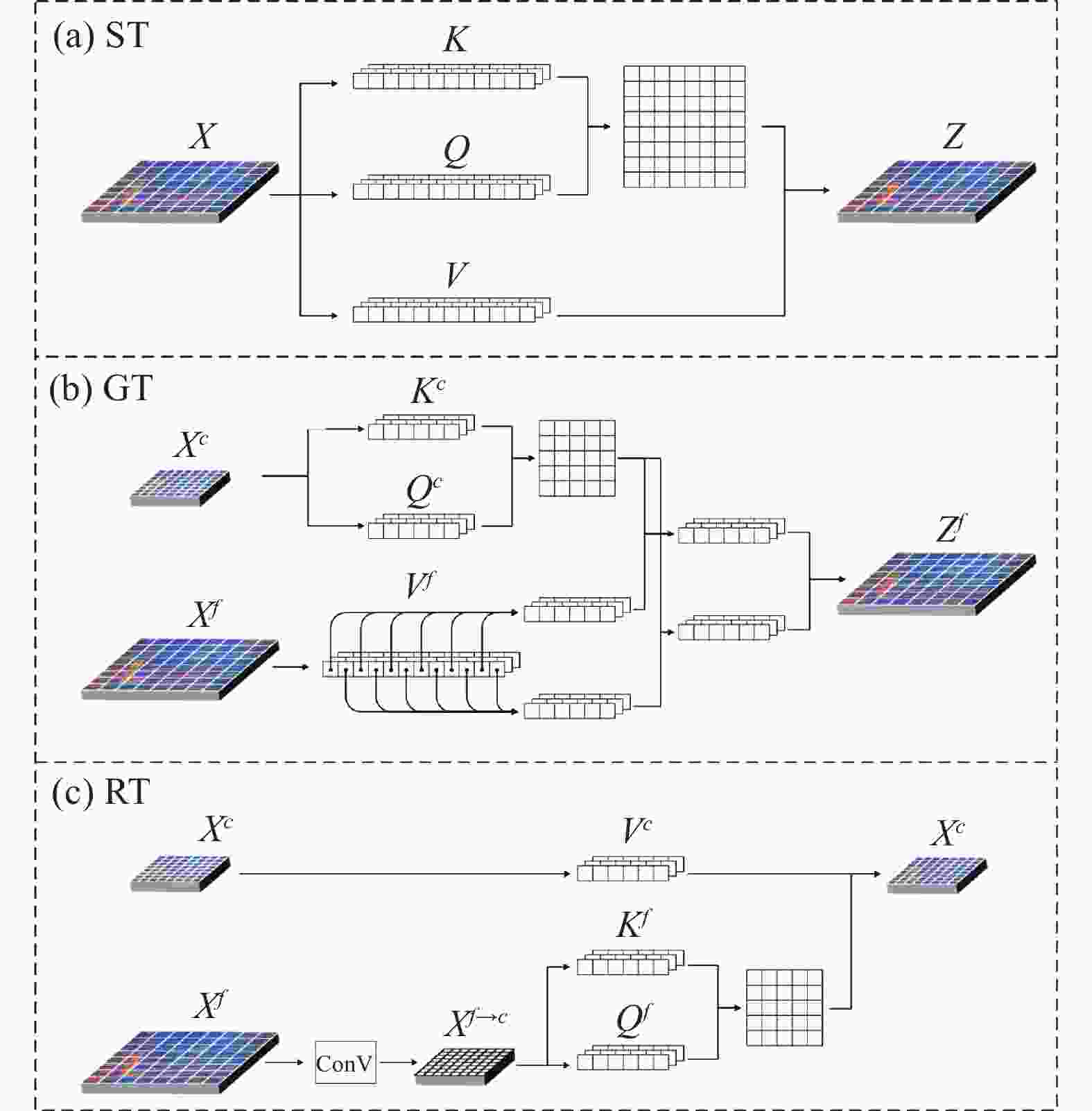

图  9  (a) ST变换；(b) GT变换；(c) RT变换

Figure 9.  (a) Self-Transformer; (b) Grounding Transformer; (c) Rendering Transformer

GT变换是高维特征矩阵${{X}}^{c}\in {\mathbb{R}}^{{d}_{c}\times {W}_{c}\times {H}_{c}}$与低维特征矩阵${{X}}^{f}\in {\mathbb{R}}^{{d}_{f}\times {W}_{f}\times {H}_{f}}$到输出矩阵$ {\textit{Z}}^{f}\in {\mathbb{R}}^{{d}_{f}\times {W}_{f}\times {H}_{f}} $的映射，如图9(b)所示，其中输出矩阵尺寸与低维特征矩阵尺寸相同。GT变换是高维特征矩阵指导低维特征矩阵变换为输出矩阵，其目的是增加低维特征图像中高维语义信息。因此，对高维特征矩阵${{X}}^{c}$进行卷积核权重为$ {W}^{Q},{W}^{K} $的1×1卷积，得到查询矩阵$ {Q}^{c} $与键矩阵$ {K}^{c} $；对低维特征矩阵${{X}}^{f}$进行卷积核权重为$ {W}^{V} $的1×1卷积，得到值矩阵$ {V}^{f} $。

GT变换的编码操作是利用查询矩阵$ {Q}^{c} $与键矩阵$ {K}^{c} $计算得到注意力矩阵$ {A}{t}{t} $。由于值矩阵$ {V}^{f}\in {\mathbb{R}}^{{d}_{f}\times {(W}_{f}\cdot {H}_{f})} $与注意力矩阵$ {A}{t}{t}\in {\mathbb{R}}^{\left({W}_{c}\cdot {H}_{c}\right)\times \left({W}_{c}\cdot {H}_{c}\right)} $维度不同，无法直接进行矩阵乘积。因此在Transformer解码操作前，需要将值矩阵$ {V}^{f} $拆解为若干子矩阵$\left\{{V}_{1}^{f},{V}_{2}^{f},\cdots ,{V}_{n}^{f}\in \right. \left. \mathbb{R}^{{d}_{f}\times \left({W}_{c}\cdot {H}_{c}\right)}\right\}$，之后将每个子矩阵分别与$ {A}{t}{t} $相乘得到子矩阵的解码输出$ \left\{{{\textit{Z}}_{1}^{f},{\textit{Z}}_{2}^{f},\cdots ,{\textit{Z}}_{n}^{f}\in \mathbb{R}}^{{d}_{f}\times \left({W}_{c}\cdot {H}_{c}\right)}\right\} $。最终将上述输出拼接为$ {\mathbb{R}}^{{d}_{f}\times {W}_{f}\times {H}_{f}} $尺寸，完成Transformer解码操作，得到GT变换的输出$ {{\textit{Z}}}^{f} $。

RT变换是低维特征矩阵$ {{X}}^{f}\in {\mathbb{R}}^{{d}_{f}\times {W}_{f}\times {H}_{f}} $与高维特征矩阵$ {{X}}^{c}\in {\mathbb{R}}^{{d}_{c}\times {W}_{c}\times {H}_{c}} $到输出矩阵$ {{\textit{Z}}}^{c}\in {\mathbb{R}}^{{d}_{c}\times {W}_{c}\times {H}_{c}} $的映射，如图9(c)所示，RT变换是低维特征矩阵增强高维特征矩阵，目的是提升小目标的判别能力。因此需要从低维特征矩阵$ {{X}}^{f} $中获取查询矩阵$ {Q}^{f} $与键矩阵$ {K}^{f} $，利用$ {Q}^{f} $与$ {K}^{f} $进行Transformer的编码操作。再从高维特征矩阵$ {{X}}^{c} $中获取值矩阵$ {V}^{c} $，值矩阵与注意力矩阵进行矩阵相乘，完成Transformer解码，得到RT变换的输出$ {{Z}}^{c} $。

由于低维特征图像尺寸大于高维特征图像，如果直接使用权重为$ {W}^{Q},{W}^{K}\in {\mathbb{R}}^{{d}_{f}\times 1\times 1} $的1×1卷积得到的查询矩阵$ {Q}^{f} $与键矩阵$ {K}^{f} $会造成编码冗余。因此在卷积前，增加一层卷积层，将$ {{X}}^{f} $转化为尺寸与$ {{X}}^{c} $相同的矩阵。

实验环境如下：操作系统采用Windows10操作系统，深度学习框架采用Pytorch1.9.1框架，CUDA11.2，网络在训练与测试时采用两张型号为NVIDIA GeForce RTX 2080的GPU，CPU型号为Intel Core i7-9700 K，64 G内存。

按8∶2的比例随机将数据集划分为训练集与验证集，训练集中包含扭转(317)、褶皱(284)、架桥(263)、气泡(201)、缺丝(84)、异物(84)；验证集中包含扭转(111)、褶皱(66)、架桥(96)、气泡(72)、缺丝(26)、异物(30)。输入网络前，使用随机翻转、随机改变对比度、随机改变亮度的操作，防止网络过拟合。模型训练周期为300个epoch，使用随机梯度下降法，初始学习率为 $ 1\times {10}^{-3} $，动量设置为0.9，学习率衰减因子 $ 5\times {10}^{-4} $，学习率分别在网络训练至150轮、200轮、250轮衰减至原来的$ 1/10 $。

在训练过程中Trans-Yolact网络损失随迭代轮数的变化如图10所示，模型在100轮内，总损失值与各部分损失值下降显著；迭代200~300轮，网络基本稳定，总损失值变化不超过$ \pm 0.5 $。可以证明采用文中方法引入Transformer后，网络可以在迭代较少轮数后稳定收敛。

图  10  Trans-Yolact网络损失

Figure 10.  Loss of Trans-Yolact

实验结果分析主要从红外与可见光联立检测的有效性、网络结构改进的有效性两方面进行论证。选择交并比为0.5时准确度AP50作为评价指标，实验P-R曲线如图11所示，实验数据见表1。在未对网络结构改进的情况下，分别测试了可见光检测、红外检测、红外与可见光联立检测三种方法。在基准Yolact网络上，仅用可见光图像检测的mAP为75.7%，仅用红外图像检测的mAP为78.8%，采用红外与可见光图像联立检测的mAP为82.5%，较可见光图像检测与红外图像检测提升6.8%、3.7%。进一步观察PR曲线可以发现，对于扭转类，采用可见光检测效果较差；架桥、气泡类，采用红外与可见光联立检测对准确度的提升较为明显。这与分析缺陷时所得结论相互印证，证明采用红外与可见光图像联立检测相比单红外或可见光图像检测更为有效。

图  11  六种复合材料缺陷的PR测试曲线

Figure 11.  PR test curves of six composite defects

对网络结构改进的有效性进行论证，文中所提出的Trans-Yolact的mAP为88.0%，相较红外与可见光图像联立检测的基准Yolact网络提升5.5%。按缺陷类别进行分析，除最易检测的架桥类缺陷外，其余种类缺陷在Trans-Yolact网络中的检测准确度均高于Yolact网络。尤其对于缺丝类、扭转类等狭长形缺陷，引入Transformer变换的Trans-Yolact网络查准率较基准网络提升15.2%、5.1%。类似的，异物类由于存在部分尺寸较大、红外与可见光图像差异明显的缺陷，Trans-Yolact网络查准率较基准网络提升9.1%。证明文中改进网络结构的方式可以有效提升对复合材料缺陷的检测效果。

为了进一步验证引入Transformer变换和改进主干网络浅层结构对网络的影响。对文中提出的Trans-Yolact网络进行消融实验，在Yolact网络基础上仅增加Transformer变换(对应2.2节与2.4节)和仅改进主干网络浅层结构(对应2.3节)进行实验。仅增加Transformer变换的网络，对缺丝类、扭转类缺陷分别提升12.1%、3.5%；对存在部分尺寸较大的异物类缺陷检测准确度提升4.9%，从正面证明引入Transformer变换可以显著提高网络从非局部空间中获取信息的能力、增强对狭长形、大尺寸缺陷的检测能力。而对于长宽近似相等的、尺寸较小的气泡类、架桥类缺陷，其检测准确度变化为−4.3%、−0.7%、，从反面证明Transformer变换对于局部小尺寸缺陷检测准确度提升不大，甚至为负作用。而仅改进主干网络浅层，对褶皱类、气泡类、异物类缺陷检测的准确度提升2.7%、2.4%、5.4%，证明对于需要综合红外与可见光信息进行判断的缺陷，从通道域对主干网络浅层的改进是有效的。但对于同样需要综合红外与可见光信息判断的架桥类缺陷，其检测准确度为93.3%，较基准网络变化−2.6%，其可能原因是架桥类缺陷检测较为容易，从红外与可见光图像检测准确度达95.9%，通道域改进对其影响不大。综上所述，文中所提出的Trans-Yolact网络增强从空间域中获取信息的能力，提升对狭长形、大尺寸缺陷的检测准确度；也增强了网络整合不同通道域信息的能力，提升网络从多源图像检测缺陷的准确度。

图12是Yolact网络与Trans-Yolact网络的效果对比，可以看出引入Transformer后，第一、四行图像中检测出未检测到的缺丝缺陷、第三行提升缺丝缺陷的检测置信度、第二行图像中检测出未检测到的扭转、气泡类缺陷、第四行提升尺寸相对较大异物缺陷的检测置信度，证明Trans-Yolact网络显著增强从非局部空间中获取信息的能力。

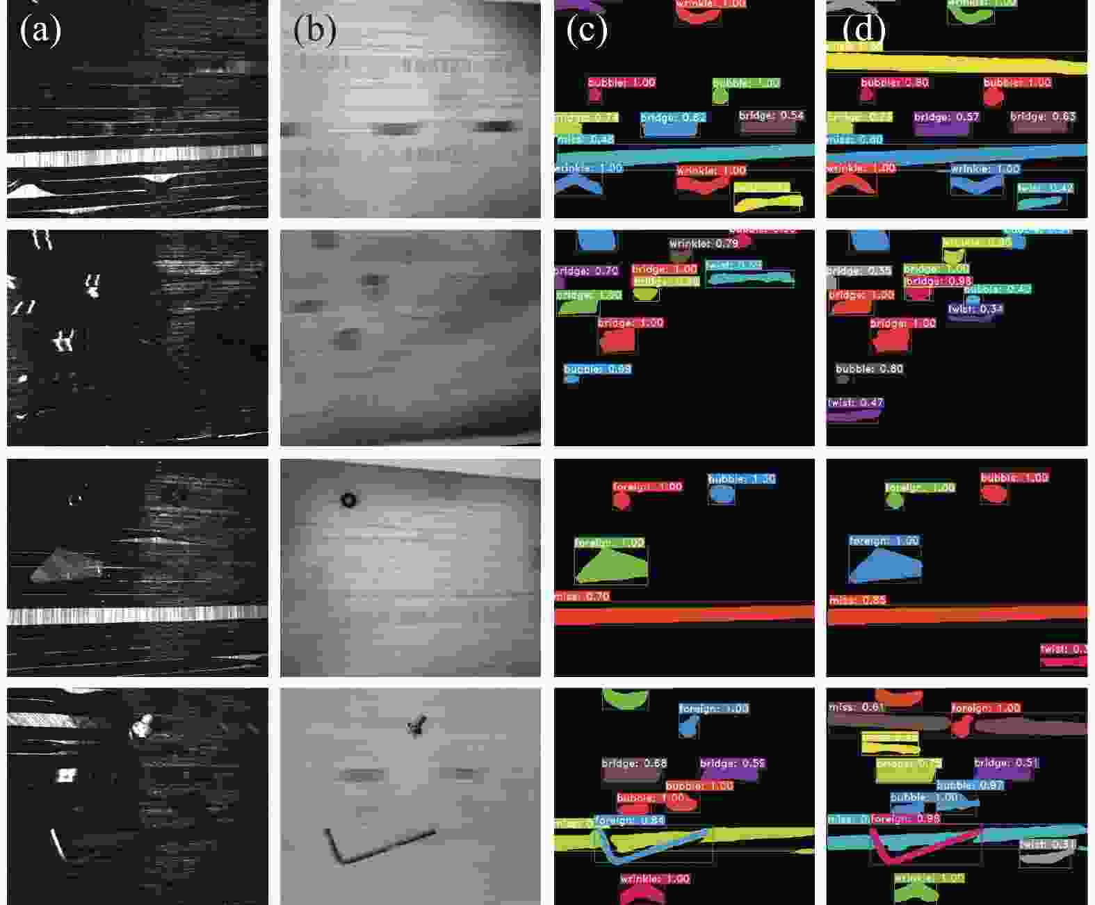
图  12  (a) 可见光图像；(b) 红外图像；(c) Yolact检测结果；(d) Trans-Yolact检测结果

Figure 12.  (a) Visible image; (b) Infrared image; (c) Yolact detection results; (d) Trans-Yolact detection results

对Trans-Yolact与Yolact进行结构化剪枝，获得一系列网络。并在复合材料缺陷数据集中对上述网络进行评估。网络结构与其对应结果如表2所示。Yolact和Trans-Yolact最大检测帧数与网络准确度的关系，如图13所示。图中圆半径代表模型所占内存大小。

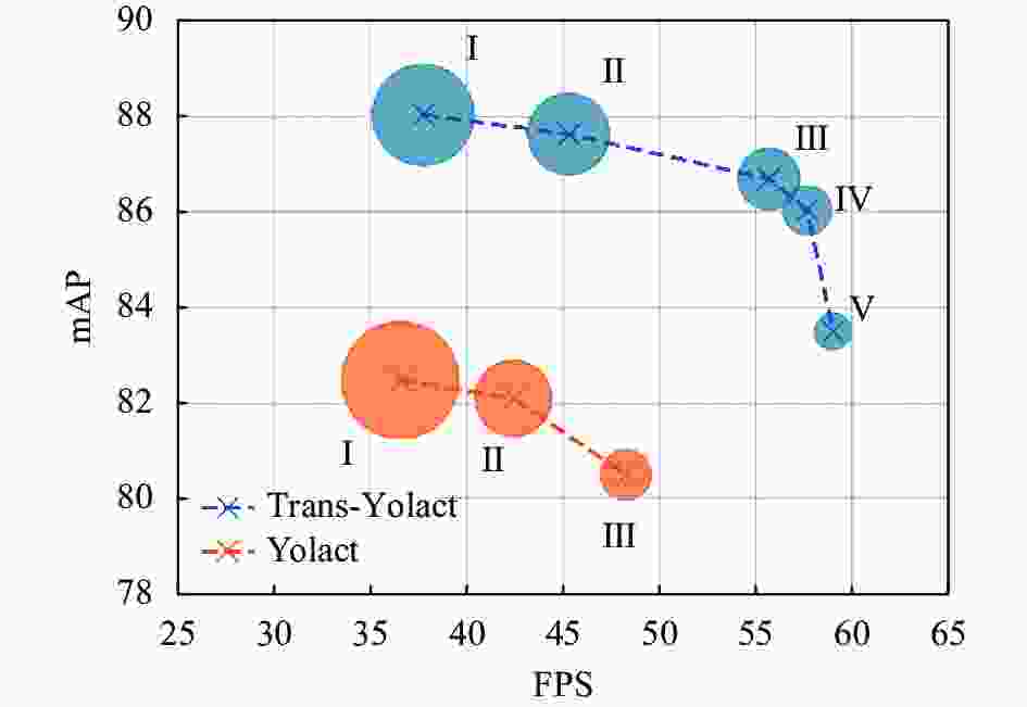
图  13  Yolact与Trans-Yolact在不同网络深度层下的实验

Figure 13.  Performance of Yolact and Trans-Yolact under different network depth layers

在对网络剪枝优化后，Trans-Yolact系列中检测速度最快的Ⅴ模型，其检测最大帧数比Yolact系列中检测速度最快的Ⅲ模型高出10 fps，达到近60 fps；Trans-Yolact系列中均衡检测精度与检测速度的Ⅳ模型，相比Yolact系列中Ⅰ模型，网络的计算量(FLOPs)减少26.5%、参数量减少44.7%、内存空间占用减少44.0%，同时检测准确度提高3.55%，检测帧数提高58%，达到57.67 fps，远超复合材料在线检测要求。可以证明，基于Transformer的Trans-Yolact，其在复合材料缺陷检测领域的表现能力优于基准Yolact网络。

最终将剪枝优化后的Trans-Yolact系列Ⅳ网络集成在复合材料实时检测软件中，在大型龙门复合材料自动铺放设备上进行在线检测测试，如图14所示。在线采集刚铺放的复合材料红外图像与可见光图像，经网络检测得到缺陷的种类、面积、轮廓掩膜等信息，利用TCP协议传输至上位机集成软件中。在线检测电脑GPU为单张Quadro 4000，检测帧数最快可达45 fps，可以满足最大铺放速度1.2 m/s下，对最小3 mm×3 mm缺陷及单股复合材料丝束缺陷的实时检测。

图  14  现场检测实验

Figure 14.  Field detecting experiment

文中提出了一种基于Transformer变换的复合材料红外与可见光联立的实例分割网络Trans-Yolact。以实时实例分割网络Yolact为基础框架，从空间域和通道域两个维度增强网络的信息整合能力。改进后Trans-Yolact网络对复合材料缺陷检测准确度可达88.0%，较基准提高5.5%。并对网络进行结构化剪枝，较基准Yolact网络减少26.5%的计算量(FLOPs)、减少44.7%的参数量；检测帧数提高58%，达到57.67 fps。最后在大型龙门复合材料自动铺放设备上进行在线测试，满足生产过程中复合材料以最大铺放速度1.2 m/s下的实时检测。并得出以下结论：

（1） 空间域上引入Transformer可以显著增强网络从非局部空间中获取信息的能力。常规卷积核具有空间尺度的局限性，文中选择CNN+Transformer结构的BoTNet作为基础主干网络、并采用基于Transformer的FPN结构。相较基准网络，Trans-Yolact网络对狭长形的缺丝类、扭转类检测准确度提升15.2%、5.1%，对含有部分大尺寸的异物类缺陷检测准确度提升9.1%。

（2）通道域上采用红外与可见光联立的检测方式，较单红外或单可见光图像mAP提高3.7%、6.8%，可以增强复合材料检测效果。在此基础上，改进主干网络浅层结构，并引入基于通道域的注意力机制(SE模块)，可以进一步提升检测准确度3.2%，增强混合通道对红外与可见光图像综合判断能力。

对复合材料缺陷进行实例分割，在得到缺陷预测框的基础上，可以获取缺陷面积、缺陷轮廓掩膜等信息，更好地辅助现场人员对复合材料缺陷进行识别，以及对复合材料构件进行产品溯源。但仍存在缺陷轮廓边缘识别模糊、铺放速度较慢时缺陷重复计数等问题，需要后续持续优化。