


-
激光雷达作为一种主动式探测的现代光学遥感技术,在目标表面快速扫描获得高精度的三维点云。目前激光雷达数据处理的研究大多集中在利用点云的几何信息实现点云的分类与特征提取[1]。激光雷达除了获取目标表面三维点云的坐标外,还测量返回的激光信号功率,反向散射的光功率在内部被转换为电压,在系统中被放大,最后被转换为DN (Digital Number)值,记录为激光后向散射强度[2],能够表征地物目标对激光脉冲发射信号的散射能力和目标辐射特性,是点云数据处理过程中重要的补充信息。
传统的激光雷达系统一般为单波长,在目标属性信息获取方面受到了单一波长的限制,激光后向散射强度数据中的光谱信息相对不足,对地物类别的探测能力有限。高光谱激光雷达作为近年来一种新型遥感探测手段,通过激光光源主动发射激光脉冲并探测后向回波的方式,提供“彩色”点云,获取被测目标的光谱信息和三维空间信息,兼具高空间探测能力与地物物理属性探测能力[3],极大地弥补了传统单波长激光雷达在地物属性辨别方面的劣势。另外,高光谱激光雷达的后向散射强度与三维坐标信息呈精确的一一对应关系,具有像素级融合的条件,无需配准,避免了传统激光雷达和高光谱遥感成像数据的融合和配准带来的额外复杂数据处理过程,也为高光谱遥感成像数据难以挖掘高精度三维信息的问题提供了可行的解决方案,具有更高的遥感应用潜力。
激光雷达后向散射强度反映了地物对激光的反射特性,有学者利用强度值进行点云分类分割、建筑物分类、土地覆盖分类等。从激光雷达后向散射强度提取目标表面或者内部某些重要特性,可以有效区分不同种类目标,如粗糙度[4]、含水量[5]、反射率、纹理、亮度等,这些是利用几何数据很难得到的,使激光雷达技术展现出更为广阔的应用[6-7],比如文化遗产、道路交通标志识别[8]、岩土层识别[9]、结构损伤检测[10]、含水量提取等。相比于传统的激光雷达系统,高光谱激光雷达系统还可以应用于地物精细分类、定量化参数反演。例如:树种精细分类、植物结构和生理信息[11]估计等。但是,在激光扫描过程中,后向散射强度受到扫描仪特性(发射功率、系统衰减、接收机孔径等)、大气衰减、目标特性、探测距离、激光入射角等因素的影响。因此,对高光谱激光雷达后向散射强度辐射特性分析和建模,消除原始强度中的各类因素的影响,使得辐射校正后的强度只与目标表面的反射特性有关,是数据充分利用的重要前提。
国内外学者对激光雷达后向散射强度强度辐射特性分析和建模的研究,可以分为四类:物理模型、半物理半经验模型、基于参考目标的方法、数据驱动方法。1)物理模型[12]基于激光传输的整个过程,在假设目标为理想朗伯体、大气条件恒定、发射的激光功率恒定的前提下,利用简化的雷达方程解释激光散射问题。这种方法具有严密的理论基础,但没有考虑实际扫描目标表面偏离理想朗伯体的影响。2)半物理半经验模型[13]是在雷达方程的物理基础上,对于非理想朗伯体,针对入射角效应,结合经验模型(例如Beckmann模型、Phong模型等)提出新的校正模型,是在各类微表面模型假设的基础上建立。3)基于参考目标的方法通过比较参考目标在实测环境和在实验室测量得到的后向散射强度数据,对目标的后向散射强度数据进行校正,也有部分方法[14]选取扫描区域中的某些自然目标(如道路)作为参考目标,抵消某些系统效应。当扫描目标与参考目标扫描几何构造相同时,入射角及距离效应也可以通过参考目标进行消除。这类方法需要事先在实验室对参考目标的激光反射特性进行测定,或者选择扫描数据中的自然目标作为参考,需要人工干预。4)数据驱动[15]的方法不考虑激光雷达工作的物理原理,基于测量得到的强度和不同的影响因素,拟合数学模型。该类模型的选取较为灵活,但没有考虑激光传输的物理背景,缺乏理论基础,估算参数依赖于数据且不稳定。
在实际应用中几乎不存在完全漫反射的目标,并且扫描对象的反射特性非常复杂,扫描对象的表面粗糙度使其偏离朗伯模型。针对粗糙表面,文中基于双向反射分布函数(Bidirectional Reflectance Distribution Function, BRDF)与雷达方程相结合,考虑目标表面的粗糙度与微小结构,基于Oren-Nayar BRDF模型,研究了高光谱激光雷达后向散射强度二向反射模型,系统性、定量化分析入射角对后向散射强度造成的影响,并基于模型实现入射角和观测角的归一化,减少同一目标由于入射角不同带来的反射率差异。为了验证模型的有效性,文中将其应用于不同粗糙度的8种目标,实验结果证明了不同目标的非朗伯特性,并定量化计算了目标的粗糙度相关参数,入射角归一化后的后向散射强度与材料的固有特性有关,与入射角无关。另外,利用构建的模型反演目标的粗糙度参数,可用于进一步的地物分类。针对文中研究的样本,基于构建的模型进行辐射校正后,不同入射角的反射率标准差不超过0.06;与校正前相比,文中方法校正后不同入射角的反射率标准差平均改进率为67.86%;所提出的模型表现出比朗伯模型更高的校正精度。该方法使得在不同激光入射角下获取的数据具有可比性,为更好地为开展高光谱激光雷达应用提供必要的物理基础。
-
激光雷达(Light Detection and Ranging, LiDAR)的工作原理与传统雷达(Radio Detection and Ranging, RADAR)相似,主要区别在于工作的波长不同。激光雷达系统发射出的激光信号经大气衰减,与目标表面发生作用,散射后再经大气作用回到激光接收机,光电探测器接收到来自目标的后向散射回波信号。激光雷达回波信号的基本原理可用雷达方程来解释说明[16],见公式(1)。设激光发射功率为$ {P}_{t} $,激光波束宽度为$\;{\beta }_{t} $,则进入接收机的总功率$ {{P}}_{{r}} $为:
$$ {P_r} = \frac{{{P_t}D_r^2}}{{4\pi {R^4}\beta _t^2}}\sigma {\eta _{atm}}{\eta _{sys}} $$ (1) 式中:$ R $为探测距离;$ {D}_{r} $为接收机孔径;考虑大气衰减和仪器衰减,$ {\eta }_{atm} $为信号在大气传输过程中的影响因子;$ {\eta }_{sys} $为激光雷达系统衰减因子;$ \sigma $为目标后向散射截面,与地物的反射特性相关,表示为:
$$ \sigma = \frac{{4\pi \rho }}{\varOmega }{A_s}\cos \theta $$ (2) 式中:$\varOmega$为目标散射的圆锥立体角;$ \;\rho $为激光雷达反射率;$ {A}_{s} $为目标的有效接收面积。当激光照射到理想的朗伯表面时,激光被均匀地散射到半球体上,即圆锥立体角等于$ \pi $的立体弧度。对于朗伯表面,激光雷达在不同角度接收的光强度与激光入射角$ \theta $ (入射光与目标表面法线的夹角)的余弦成正比。此时,激光雷达散射截面表示为:
$$ \sigma = \pi {R^2}\beta _t^2\rho \cos \theta $$ (3) 带入雷达方程,可得朗伯体目标雷达方程为:
$$ {P_r} = \frac{{{P_t}D_r^2\rho \cos \theta }}{{4{R^2}}}{\eta _{atm}}{\eta _{sys}} $$ (4) 设中心波长为$ \mathrm{\lambda } $,在高光谱激光雷达系统设计的不同光谱的发射和探测接收系统参数一致的情况下,朗伯体目标高光谱激光雷达不同波长的接收功率可以写为:
$$ {P_r}(\lambda ) = \frac{{{P_t}(\lambda )D_r^2\rho (\lambda )\cos \theta }}{{4{R^2}}}{\eta _{atm}}(\lambda ){\eta _{sys}}(\lambda ) $$ (5) 式中:$ {P}_{r}\left(\lambda \right) $是传感器在高光谱激光雷达系统的特定激光波长$ \lambda $下的总接收功率。
假设物体表面具有朗伯散射特性,在一次测量过程中大气条件是恒定的。在激光扫描过程中,$ {P}_{t}\left(\lambda \right) $,$ {D}_{r} $,$ {\eta }_{atm}\left(\lambda \right) $和$ {\eta }_{sys}\left(\lambda \right) $可以看作是四个常数。通常,后向散射强度$ \mathrm{I}\left(\mathrm{\lambda }\right) $与接收功率$ {P}_{r}\left(\lambda \right) $正相关。因此,公式(5)可以推导为:
$$ I(\lambda ) = \frac{{C(\lambda )\rho (\lambda )\cos \theta }}{{{R^2}}} $$ (6) 式中:$ C\left(\lambda \right) $可以看作常数。因此,对于理想的朗伯表面,高光谱激光雷达不同波长的后向散射强度与$ \cos \theta $成正比,与$ {R}^{2} $成反比。在许多应用中,入射角效应和距离效应是叠加在一起的综合效应。由公式(6)可以看出,距离效应和入射角效应相互独立。
针对同一个目标,假设激光扫描过程中入射角恒定,高光谱激光雷达不同波长的后向散射强度与$ {R}^{2} $成反比。高光谱激光雷达距离效应辐射校正如公式(7)所示。其中$ I(R,\lambda ) $为探测距离为$ R $和波长为$ \lambda $时的后向散射强度,$ {R}_{s} $为标准距离,$ {I(R,\lambda )}_{c} $为辐射校正到标准距离的后向散射强度。
$$ I{(R,\lambda )_c} = I(R,\lambda ) \cdot \frac{{{R^2}}}{{R_s^2}} $$ (7) 假设激光扫描过程中距离恒定,则对于理想的朗伯表面,高光谱激光雷达不同波长的后向散射强度与$ \cos \theta $成正比。如公式(8)所示:
$$ I{(\theta ,\lambda )_s} = {f_0}(\lambda )\cos \theta $$ (8) 式中:$ {f}_{0}\left(\lambda \right) $为法线方向的后向散射强度;$ I{\left(\theta ,\lambda \right)}_{s} $为入射角为$ \theta $和波长为$ \lambda $时的后向散射强度。
-
在真实环境中扫描对象的反射特性复杂,在实际应用中几乎不存在完全漫反射的目标,扫描目标的表面粗糙度使得扫描对象的反射特性偏离朗伯模型,因此粗糙地物与激光脉冲的相互作用非各向同性,而是具有方向性,利用朗伯模型表征入射角效应是不够的。
Nayar等人[17]1991年在计算机图形学领域中提出的光反射模型——Oren-Nayar模型。Oren-Nayar模型是一个模拟粗糙表面漫反射的物理反射模型,该模型预测粗糙表面在光源方向上比朗伯表面返回更多的光。粗糙表面是指目标表面上具有的较小间距和峰谷所组成的微观几何形状特性,可以被建模为一系列不同朝向的微小平面的集合,每一个微小平面可以看成是一个漫反射平面。
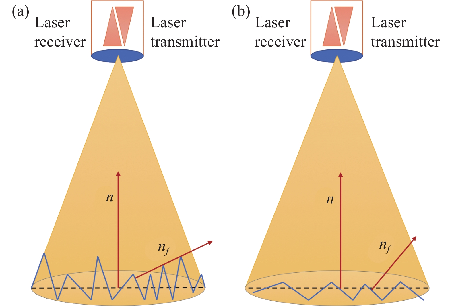
如图1所示,通过 “V” 形微面描述粗糙表面,微表面的法线方向$ {n}_{f} $方差越大,宏观表面越粗糙;微表面的法线方向$ {n}_{f} $方差越小,宏观表面越光滑。当所有的微小平面组合起来后,其反射特性明显偏离朗伯反射。与朗伯模型相比,Oren-Nayar模型考虑了目标表面的粗糙度与微小结构,更加符合真实自然目标的激光反射情况。

图 1 (a) 微表面的法线方差越大,宏观表面越粗糙;(b) 微表面的法线方差越小,宏观表面越光滑
Figure 1. (a) The larger the variance of the normal direction of the micro surface, the rougher the macro surface; (b) The smaller the variance of the normal direction of the micro surface, the smoother the macro surface
Oren-Nayar模型是双向反射分布函数,对入射方向和出射方向对辐亮度进行建模,根据该模型,出射方向的辐亮度表示为:
$$ \begin{split} L =& \rho {E_0}\cos \alpha \times\\ & (A + B {\rm{Max}} [0,\cos ({\phi _r} - {\phi _i})]\sin \alpha \tan \beta ) \\ \end{split} $$ (9) $$ {{A}} = 1 - 0.5\frac{{{\sigma ^2}}}{{{\sigma ^2} + 0.33}} $$ (10) $$ {{B}} = 0.45\frac{{{\sigma ^2}}}{{{\sigma ^2} + 0.09}} $$ (11) 式中:$ {E}_{0} $为以法向方向接收的辐射通量;$ \;\rho $为目标的反射率;$ \alpha $为入射角;$\; \beta $为出射角;$ {\phi }_{i} $为入射方向的方位角;$ {\phi }_{r} $为出射方向的方位角;$ \sigma $为微小平面坡角分布的标准差,取值范围是 [0°, 90°]。
对于激光雷达系统,激光发射与激光接收位置重合。因此,$ \alpha =\beta $,$ \mathrm{cos}\left({\phi }_{r}-{\phi }_{i}\right)=1 $。Oren-Nayar模型简化为:
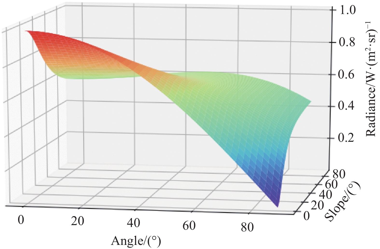
$$ L = \rho {E_0}\cos \alpha (A + B\sin \alpha \tan \beta ) $$ (12) $$ {{A}} = 1 - 0.5\frac{{{\sigma ^2}}}{{{\sigma ^2} + 0.33}} $$ (13) $$ {{B}} = 0.45\frac{{{\sigma ^2}}}{{{\sigma ^2} + 0.09}} $$ (14) 设定$\; {\rho E}_{0} $为1,$ \sigma $取不同值时,Oren-Nayar模型出射方向的辐亮度随$ \sigma $和入射角的变化趋势如图2所示。图中的Slope表示为微小平面坡角分布的标准差$ \sigma $,单位为度;Angle为入射角,单位为度;Radiance为辐亮度,单位为$\mathrm{W}/\left({\mathrm{m}}^{2}\cdot \mathrm{s}\mathrm{r}\right)$。由图2可以看出,$ \sigma $对于$ L $的影响较大,$ \sigma $越大,出射方向的辐亮度越偏离朗伯模型。

图 2 Oren-Nayar模型示意图
Figure 2. Schematic diagram of Oren-Nayar model
-
对于高光谱激光雷达,设不同波长为$ \lambda $,基于Oren-Nayar模型改进后的粗糙表面二向反射模型为:
$$ I(\theta ,\lambda ) = {f_0}(\lambda )\cos \theta (A(\lambda ) + B(\lambda )\sin \theta \tan \theta ) $$ (15) $$ {{A}}(\lambda ) = 1 - 0.5\frac{{\sigma {{(\lambda )}^2}}}{{\sigma {{(\lambda )}^2} + 0.33}} $$ (16) $$ {{B}}(\lambda ) = 0.45\frac{{\sigma {{(\lambda )}^2}}}{{\sigma {{(\lambda )}^2} + 0.09}} $$ (17) 式中:$ I(\theta ,\lambda ) $为波长为$ \lambda $和入射角为$ \theta $时的后向散射强度;$ {f}_{0}\left(\lambda \right) $为法线方向的后向散射强度;$ \sigma \left(\lambda \right) $为波长为$ \lambda $时的微小平面坡角分布的标准差,取值范围是 [0°, 90°]。
对于同一个粗糙表面,微小平面坡角分布的标准差在不同的波段是相同的,因此,文中定义该表面统一的$ {\sigma }_{mean} $为不同波长的$ \sigma \left(\lambda \right) $的平均值:
$$ {\sigma _{mean}} = \sqrt {\frac{{\displaystyle\sum\limits_{i = 1}^n {{\sigma ^2}({\lambda _n})} }}{n}} $$ (18) 式中:n为波段数。对于$ {\mathrm{\sigma }}_{mean} $越小的平坦表面,Oren-Nayar模型越接近朗伯模型。
根据公式(11),文中提出了对于粗糙表面高光谱激光雷达后向散射强度的入射角效应辐射校正模型:
$$ I{(\theta ,\lambda )_c} = \frac{{I(\theta ,\lambda )\cos {\theta _s}}}{{\cos \theta ({A_{mean}} + {B_{mean}}\sin \theta \tan \theta )}} $$ (19) $$ {{{A}}_{mean}} = 1 - 0.5\frac{{{\sigma _{mean}}^2}}{{{\sigma _{mean}}^2 + 0.33}} $$ (20) $$ {{{B}}_{mean}} = 0.45\frac{{{\sigma _{mean}}^2}}{{{\sigma _{mean}}^2 + 0.09}} $$ (21) 式中:$ {I(\theta ,\lambda )}_{c} $是波长为$ \lambda $和入射角为$ \theta $时校正后的后向散射强度;$ I(\theta ,\lambda ) $是波长为$ \lambda $和入射角为$ \theta $时原始实测的后向散射强度;$ {\theta }_{s} $为标准入射角,该模型不同入射角的后向散射强度都归一化到$ {\theta }_{s} $的入射角。
-
高光谱激光雷达系统[18-20]主要包括激光发射单元、激光接收单元、扫描和控制单元等关键部件。
激光发射单元主要由超连续谱激光器、声光可调谐滤波器、准直扩束器和反射镜组成。采用超连续谱激光器作为光源,持续发出超连续谱激光,经声光可调谐滤波器(Acousto-optic Tunable Filter,AOTF)调谐滤波后在不同时刻发射不同波长单色光。AOTF通过时间域上的信号调谐选择不同波长。激光扩束器主要用来调节激光光束,对其进行准直,减小其发散角,将其变为平行光束,确保发射能量的集中。反射镜的主要作用是将调谐后的单色激光经过45°偏转后发射到探测目标上。
激光回波信号接收单元主要由接收光学系统、光电探测器、数据采集系统等组成,其作用是通过望远光学系统将激光回波信号收集到光电探测器上,激光探测器将光信号转为电信号,通过放大电路进行放大,并由数据采集系统完成模数转换和信息采集,将高光谱激光雷达全波形回波信号记录下来。
激光扫描控制单元的主要作用是对发射系统的发射光束和接收系统的瞬时接收视场方向进行同步扫描和控制。发射和接收光学系统整体搭载于二维转台,实现水平、垂直两个方向的扫描。系统综合控制软件主要负责控制激光器、滤波器、二维转台和数据采集卡协同工作并保障数据之间的匹配关系。
该研究主要使用中国科学院定量遥感信息技术重点实验室已有的一套自行研制的基于AOTF可调谐高光谱激光雷达原理样机[18-20],系统的组成如图3(a)所示,原理样机如图3(b)所示。

图 3 高光谱激光雷达仪器。(a) 高光谱激光雷达系统的组成图;(b) 高光谱激光雷达原理样机
Figure 3. Hyperspectral LiDAR system. (a) Composition diagram of hyperspectral LiDAR system; (b) Principle prototype of hyperspectral LiDAR
该系统选择SC-OEM作为超连续谱光源,光谱宽度为400~2400 nm,可提供重复频率为0.1~200 MHz。选用的AOTF滤波器型号为AOTF-PRO定制版,其波长输出范围覆盖530~900 nm超宽波段,光谱分辨率1~10 nm。接收光学系统选用了型号为APD210的硅雪崩光电探测器作为接收元件,接收的波长范围是400~1 000 nm。激光雷达的回波信号采集由一块数据采集卡完成,采样率为10 GPS。
-
为验证该研究提出的针对粗糙表面的二向反射模型,并分析高光谱激光雷达后向散射强度与激光入射角之间的关系,有针对性地选择了不同粗糙度的朗伯体样本作为探测目标,如图4所示。实验样本共有8种目标,分别是3种常见地物和5种矿石样本:白纸、地砖、混凝土、石膏、正长石、硅石、花岗岩、大理岩。其中,白纸为办公用的A4纸,是8种目标中最光滑的。其他7种目标均有明显粗糙的表面。

图 4 实验样本。(a)白纸;(b)地砖;(c)混凝土;(d)石膏;(e)正长石;(f)硅石;(g)花岗岩;(h)大理岩
Figure 4. Experimental sample. (a) White paper; (b) Floor tiles; (c) Concrete; (d) Gypsum; (e) Orthoclase; (f) Silica; (g) Granite; (h) Griotte
建立一个测角平台实现不同激光入射角的探测方式,高光谱激光雷达的位置和激光发射方向不变,通过水平旋转目标改变激光入射角,如图3(a)所示。平台上固定一个量角器来显示目标旋转的角度作为激光入射角。目标探测距离大约为4 m。入射角的变化范围是0°~70°,以10°为增量步长。入射角实验中,文中选择信噪比较优的波段范围进行实验,排除噪声带来的影响。因此,激光探测的波段范围设置为650~850 nm,采样步长为10 nm,共计21个波长。实验过程中,记录了每个波长和每个入射角的50次后向散射强度,取平均值作为强度结果以增加最终的信噪比。
使用具有相同探测距离的100%标准参考板计算目标的反射率$ \;\rho \left(\lambda \right) $,如公式(14)所示:
$$ \rho (\lambda ) = \frac{{{I_{tar}}(\lambda )}}{{{I_{ref}}(\lambda )}}{\rho _{ref}}(\lambda ) $$ (22) 式中:$ {I}_{ref}\left(\lambda \right) $是标准反射板的后向散射强度;$ {I}_{tar}\left(\lambda \right) $是探测目标的后向散射强度;$\;{\rho }_{ref}\left(\lambda \right) $是标准反射板的反射率。
-
文中使用的高光谱激光雷达的工作距离至少为3.3 m。因此,在实验室条件下,以100%和70%标准漫反射板为目标垂直入射(入射角为0°),改变目标到激光雷达的传输距离(步长为1 m),采集了传输距离为4~20 m的后向散射强度,实验过程如图5所示。激光探测的波段范围同样设置为650~850 nm,采样步长为10 nm,共计21个波长。

图 5 距离效应实验示意图
Figure 5. Schematic diagram of distance effect experiment
-
为了分析具有不同反射特性和粗糙度目标的入射角效应,绘制了不同样本后向散射强度随入射角变化的曲线。图6显示了8个实验样本在不同波长下的入射角效应,横轴为激光入射角,单位为(°);纵轴为后向散射强度,单位为V。

图 6 高光谱激光雷达不同波段后向散射强度入射角效应。(a) 白纸;(b)地砖;(c) 混凝土;(d)石膏;(e)正长石;(f)硅石;(g)花岗岩;(h)大理岩
Figure 6. Incident angle effect of backscatter intensity of hyperspectral LiDAR at different wavelengths. (a) White paper; (b) Floor tiles; (c) Concrete; (d) Gypsum; (e) Orthoclase; (f) Silica; (g) Granite; (h) Griotte
可以看出,激光入射角对原始记录的后向散射强度有显著影响,强度随着入射角的增加而减小。对于白纸样本,21个波长的后向散射强度随入射角变化的曲线呈现出类似余弦函数的趋势。但是,其他样本的变化趋势不同程度偏离朗伯模型。以地砖和混凝土为例,文中绘制了在650 nm时后向散射强度的散点图(红色点)和朗伯模型拟合曲线(绿色虚线)的比较,如图7所示。

图 7 波段为650 nm的后向散射强度的散点图和朗伯模型拟合曲线对比图。(a) 地砖;(b) 混凝土
Figure 7. Scatter plot and Lambertian model fitting curve of backscatter intensity (650 nm). (a) Floor tiles; (b) Concrete
由图7可以看出,对于地砖和混凝土这两种粗糙目标,入射角较小时,其规律接近余弦函数趋势,入射角越大,尤其是在40°后,明显偏离朗伯模型的拟合曲线。
-
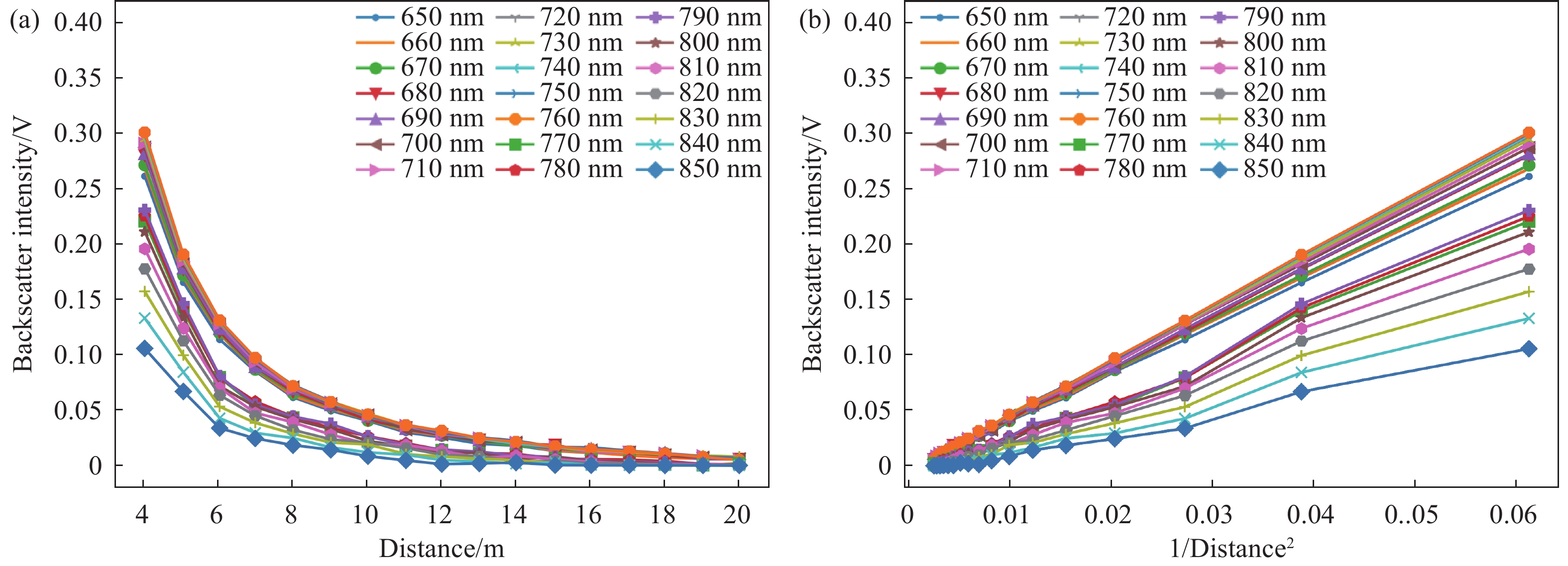
为了分析目标的入射角效应,文中绘制了100%和70%漫反射板的后向散射强度随探测距离R变化的曲线,分别如图8(a)和图9(a)所示。其中,横轴为激光探测距离,单位为m;纵轴为后向散射强度,单位为V。由公式(7)可得,后向散射强度与探测距离的平方成反比。图8(b)和图9(b)分别绘制了两种目标的后向散射强度随$ 1/{R}^{2} $的变化曲线。

图 8 100%漫反射板的不同波段后向散射强度的距离效应。(a) 后向散射强度随探测距离R变化的曲线;(b) 后向散射强度随$ 1/{R}^{2} $变化的曲线
Figure 8. Distance effect of backscatter intensity of 100% diffuse reflective whiteboard at different wavelengths. (a) The curve of the backscatter intensity varying with R; (b) Curve of backscatter intensity varying with $ 1/{R}^{2} $

图 9 70%漫反射板的不同波段后向散射强度的距离效应。(a) 后向散射强度随探测距离R变化的曲线;(b) 后向散射强度随$ 1/{R}^{2} $变化的曲线
Figure 9. Distance effect of backscatter intensity of 70% diffuse reflective whiteboard at different wavelengths. (a) The curve of the backscatter intensity varying with R; (b) Curve of backscatter intensity varying with $ 1/{R}^{2} $
由图8和图9可以看出,100%和70%漫反射板两个目标的后向散射强度与探测距离$ {R}^{2} $成反比,与$ {1/R}^{2} $线性相关,变化规律符合公式(6)和公式(7)。
-
使用公式(11)中的模型对每个波长和每个样本进行非线性曲线拟合,并使用最小二乘法计算不同波长的参数$ \mathrm{\sigma }\left(\mathrm{\lambda }\right) $,参数$ \mathrm{\sigma }\left(\mathrm{\lambda }\right) $(图中用Slope表示,单位为(°))和不同波长$ \mathrm{\lambda } $之间的关系计算结果如图10所示。参数$ \mathrm{\sigma }\left(\mathrm{\lambda }\right) $在不同波长的计算结果比较稳定,由公式(12)计算得到每种样本的平均参数$ {\mathrm{\sigma }}_{mean} $,如表1所示。

图 10 Oren-Nayar模型不同样本的参数$ {\sigma }\left({\lambda }\right) $的计算结果
Figure 10. Calculation results of $ {\sigma }\left({\lambda }\right) $ of different samples of Oren-Nayar model
表 1 Oren-Nayar模型不同样本的σmean计算结果
Table 1. σmean calculation results of different samples of Oren-Nayar model
No. Target ${\mathrm{\sigma } }_{mean}$/(°) 1 White paper 0.008 2 Floor tiles 13.93 3 Concrete 15.67 4 Gypsum 11.31 5 Orthoclase 7.56 6 Silica 5.30 7 Granite 12.81 8 Griotte 5.71 对于实验中的白纸样本,$ {\mathrm{\sigma }}_{mean} $接近于0,表明其几乎接近朗伯体。对于实验中的其他样本,都具有明显的粗糙度,$ {\mathrm{\sigma }}_{mean} $取值均大于 5°,与图6中的分布曲线对比可以看出,$ {\mathrm{\sigma }}_{mean} $越大,不同波段后向散射强度入射角效应越偏离朗伯模型。混凝土的$ {\mathrm{\sigma }}_{mean} $最大,与样本的实际粗糙度和光学反射特性一致。
-
根据公式(13)和拟合模型参数$ {\mathrm{\sigma }}_{mean} $,将不同入射角的反向散射强度归一化到垂直入射角度(0°)。研究中所有样品的校正后的后向散射强度随入射角变化曲线如图11所示,横轴为激光入射角,单位为(°);纵轴为后向散射强度,单位为V。图11表明同一样本在相同波长下,校正后的强度是近似的。
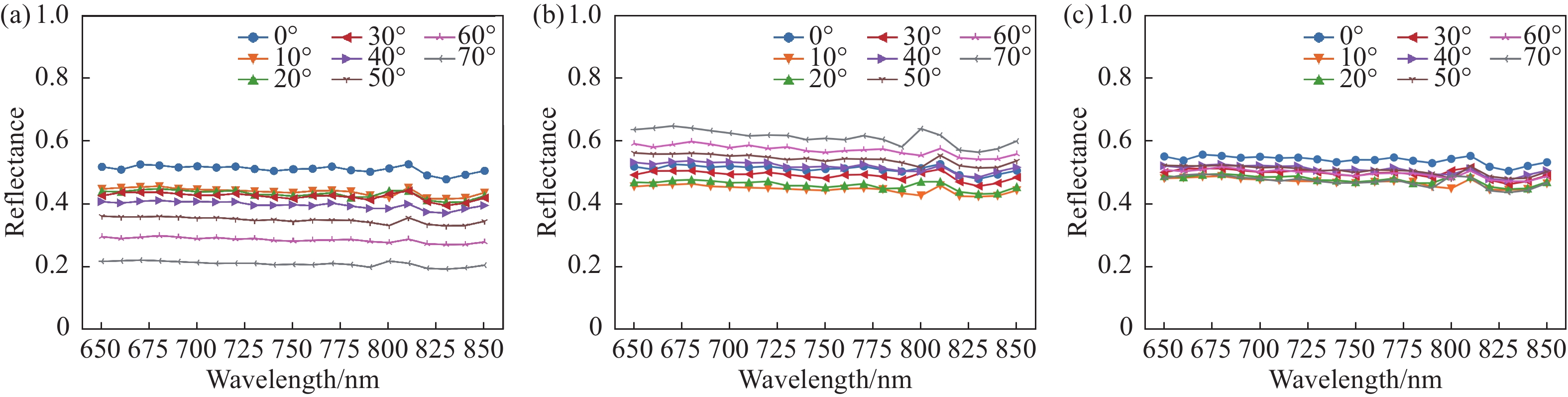
为了验证研究中提出的辐射定标模型的可行性,文中选择混凝土样本,计算并比较了校准前后的反射率和基于朗伯模型校正的反射率,如图12所示,横轴为波长,纵轴为反射率。尽管同一目标有相同的散射特性,但是在校正前的不同入射角情况下,反射率显著不同。在校正前不同入射角的反射率曲线分布是离散的,基于朗伯模型校正后反射率的分布相对集中,Oren-Nayar模型校正后反射率曲线的分布更集中。研究的方法可以显著降低入射角对反射率的影响。
以上结果都表明了所提出的后向散射强度二向性反射模型的可行性。为了进一步定量证明研究方法的有效性,文中计算并对比了校正前后及基于朗伯模型校正后,各个波段反射率在不同入射角下的标准差的散点对比图,如图13所示,其中横轴为波长,单位为nm;纵轴为标准差。所有波段的反射率标准差的平均值如表2所示。

图 11 Oren-Nayar模型校正后校正后不同波段的后向散射强度随角度变化。(a) 白纸;(b)地砖;(c) 混凝土; (d)石膏;(e)正长石;(f)硅石;(g)花岗岩;(h)大理岩
Figure 11. Backscatter intensity of different wavelengths after correction of Oren-Nayar model. (a) White paper; (b) Floor tiles; (c) Concrete; (d) Gypsum; (e) Orthoclase; (f) Silica; (g) Granite; (h) Griotte

图 12 混凝土样本在校正前后不同入射角反射率的对比。(a) 校正前;(b)朗伯模型校正后;(c) Oren-Nayar模型校正后
Figure 12. Reflectance comparison of different incident angles before and after correction of concrete. (a) Before correction; (b) After correction of Lambert model; (c) After correction of Oren-Nayar model

图 13 各个波段的反射率在不同入射角的标准差。(a) 白纸;(b)地砖;(c) 混凝土;(d)石膏;(e)正长石;(f)硅石;(g)花岗岩;(h)大理岩
Figure 13. Standard deviation of reflectance at different incident angles. (a) White paper; (b) Floor tiles; (c) Concrete; (d) Gypsum; (e) Orthoclase; (f) Silica; (g) Granite; (h) Griotte
表 2 所有波段的反射率在不同入射角的标准差平均值
Table 2. Average value of standard deviation of reflectance at different incident angles
No. Target Before correction Correction of Lambertian model Correction of Oren-Nayar model 1 White paper 0.260 0.060 0.060 2 Floor tiles 0.041 0.061 0.016 3 Concrete 0.055 0.143 0.040 4 Gypsum 0.096 0.056 0.024 5 Orthoclase 0.111 0.058 0.029 6 Silica 0.126 0.037 0.024 7 Granite 0.064 0.070 0.016 8 Griotte 0.144 0.060 0.039 分析校正结果后,可以得出以下结论:
1)对于白纸样本,$ {\mathrm{\sigma }}_{mean} $接近0,Oren-Nayar等价于朗伯模型,其校正效果后的标准差和朗伯模型相同,朗伯模型和Oren-Nayar模型校正后的标准差的散点几乎重合。对于粗糙度较小的目标,$ {\mathrm{\sigma }}_{mean} $越小,Oren-Nayar模型校正结果越接近朗伯模型。
2)对于具有明显粗糙度的样品,Oren-Nayar模型校正后的效果提升很大,可以明显地消除入射角效应,尤其是对于粗糙度越大的目标。针对文中研究的样本,基于构建的模型进行辐射校正后,不同入射角的反射率标准差的均值都不超过0.06。与校正前相比,文中方法校正后不同入射角的反射率标准差平均改进率为67.86%。其中,硅石的改进率最大,为80.95%。
3)对于地砖、混凝土和花岗岩,这类样本的$ {\mathrm{\sigma }}_{mean} $均大于10°,朗伯模型校正后的标准差大于校正前的标准差。说明朗伯模型的校正方法不适用于粗糙度大的目标。
4)基于文中提出的模型,自适应地计算了目标的粗糙度。模型将不同入射角的后向散射强度归一化到法线入射方向,结果可用于进一步的目标分类,同时粗糙度也可以作为进一步提高分类精度的重要特征。
-
高光谱激光雷达的后向散射强度代表了目标对发射激光束后向散射回波的光功率,能够表征目标的辐射特性。为了更准确地获取目标的后向散射强度,研究针对粗糙表面,分析了高光谱激光雷达后向散射强度与入射角的关系,将Oren-Nayar模型与雷达方程相结合,构建了考虑目标粗糙度的二向反射模型。通过定量化计算粗糙表面的微小平面坡角分布的标准差,建立精确的二向反射模型,将不同入射角的后向散射强度校正到法线方向,有效地消除入射角对反射率的影响。
研究选择典型的8种粗糙样品进行实验,不同入射角的实验结果表明,高光谱激光雷达的后向散射强度并不完全遵循朗伯模型。对于粗糙度较大的目标,微小平面坡角分布的标准差越大,越偏离朗伯模型。与朗伯模型的校正方法相比,所提出的模型具有更高的校正精度,实验中样本的最大改进率为80.95%,研究中样品的平均改进率为67.86%。进一步为提高基于高光谱激光雷达的点云分割和分类的精度开辟新的前景,同时对粗糙度的定量化计算也为点云的特征提取提供新的思路。
在高光谱激光雷达的扫描过程中,后向散射强度受到许多因素的影响,如仪器系统的特性、距离、环境等。未来,笔者将进一步研究高光谱激光雷达系统特性、环境等因素的影响,构建更综合的后向散射强度辐射校正模型。
Bidirectional reflectance distribution function model of rough surface based on backscatter intensity of hyperspectral LiDAR
-
摘要: 高光谱激光雷达是同时获取光谱和空间信息的主动遥感探测方法。在激光扫描过程中,激光入射角是重要的影响因素之一。在实际应用中,目标表面粗糙度会使其入射角效应偏离朗伯模型。因此,基于Oren-Nayar模型对粗糙表面建立二向反射模型,研究了入射角效应的辐射校正方法。选取8种典型的粗糙表面作为实验对象,分析了各波段后向散射强度与入射角的关系,并量化了粗糙度对强度的影响。基于构建的模型,对该研究样本的入射角效应进行辐射校正。辐射校正后,不同入射角反射率的标准差均不大于0.06;与校正前相比,标准差平均改善率为67.86%。结果表明,所提出的方法提高了提取目标反射特性的准确性,为高光谱激光雷达更好地为开展数据分析与应用提供良好的物理基础。Abstract:
Objective The traditional LiDAR system operates at a single wavelength, which limits the acquisition of target attribute information. The spectral information captured by laser backscatter intensity is relatively insufficient, and the detection ability of ground object categories is also limited. Hyperspectral LiDAR, on the other hand, is an active remote sensing method that can obtain spectral and spatial information of targets simultaneously. In addition to 3D coordinates, hyperspectral LiDAR also records the backscatter intensity of each point, enabling the detection of the geometric and reflection characteristics of targets. However, the backscatter intensity of the laser is affected by multiple factors during scanning, making it unsuitable for directly reflecting the reflection characteristics of the target surface. One of the most crucial factors is the laser incidence angle. In practical applications, there are few complete Lambertian targets, and the reflection characteristics of the scanned objects are very complex. Moreover, the roughness of the scanned target deviates from the Lambertian model. Therefore, considering the roughness and micro-structure of the target surface, this study proposes a BRDF model for rough surfaces based on the backscatter intensity of hyperspectral LiDAR through the combination of bidirectional reflection distribution function (BRDF) and radar equation. Methods This paper proposes a BRDF model based on the Oren-Nayar model for rough surfaces to address the effect of incident angle on the backscatter intensity data of hyperspectral LiDAR. The hyperspectral LiDAR system comprises key components such as a laser transmitting unit, a laser receiving unit, a scanning and control unit. By combining theory with experiments, eight typical rough targets were selected to analyze the relationship between backscatter intensity and incident angle of hyperspectral LiDAR and quantify the effect of surface roughness on intensity. The radiometric correction method for the incident angle effect was studied based on the constructed model. Results and Discussions The incident angle of the laser has a significant effect on the backscatter intensity of the original record, and the intensity decreases with the increase of the incident angle. For the white paper sample, the curve of the backscatter intensity of 21 wavelengths with the incident angle shows a trend similar to the cosine function. However, the changing trend of other samples deviates from the Lambertian model to varying degrees. After radiometric correction based on the constructed model, the standard deviation of reflectance at different angles was no more than 0.06, and the average improvement rate of the standard deviation was 67.86% compared to before correction. The proposed model exhibited higher correction accuracy than the Lambertian model. The results show that the proposed method successfully eliminates the influence of the incident angle of hyperspectral LiDAR. Conclusions In this study, we analyze the relationship between the backscatter intensity of hyperspectral LiDAR and the incident angle for rough surfaces. We construct a BRDF model that considers target roughness by combining the Oren-Nayar model with the radar equation. By quantitatively calculating the standard deviation of the slope of the rough surface, we establish an accurate radiometric correction model. This correction model enables us to effectively eliminate the impact of incident angles on reflectance. We selected eight typical rough samples for experiments and obtained experimental results at different incident angles. These results show that the backscatter intensity of the hyperspectral LiDAR does not completely follow the Lambertian model, especially for targets with large roughness. The larger the standard deviation of the slope is, the more the backscatter intensity deviates from the Lambertian model. The proposed correction model offers higher accuracy compared to the Lambertian model. The maximum improvement rate of the sample in the experiment is 80.95%, and the average improvement rate for all samples is 67.86%. Our study opens up new prospects for improving the accuracy of point cloud segmentation and classification based on the hyperspectral LiDAR. The quantitative calculation of roughness also provides new ideas for feature extraction of point clouds. This proposed method offers an effective solution for the radiometric correction of incident angle effects of hyperspectral LiDAR and provides a good physical basis for data analysis and application. -
图 1 (a) 微表面的法线方差越大,宏观表面越粗糙;(b) 微表面的法线方差越小,宏观表面越光滑
Figure 1. (a) The larger the variance of the normal direction of the micro surface, the rougher the macro surface; (b) The smaller the variance of the normal direction of the micro surface, the smoother the macro surface
图 3 高光谱激光雷达仪器。(a) 高光谱激光雷达系统的组成图;(b) 高光谱激光雷达原理样机
Figure 3. Hyperspectral LiDAR system. (a) Composition diagram of hyperspectral LiDAR system; (b) Principle prototype of hyperspectral LiDAR
图 4 实验样本。(a)白纸;(b)地砖;(c)混凝土;(d)石膏;(e)正长石;(f)硅石;(g)花岗岩;(h)大理岩
Figure 4. Experimental sample. (a) White paper; (b) Floor tiles; (c) Concrete; (d) Gypsum; (e) Orthoclase; (f) Silica; (g) Granite; (h) Griotte
图 6 高光谱激光雷达不同波段后向散射强度入射角效应。(a) 白纸;(b)地砖;(c) 混凝土;(d)石膏;(e)正长石;(f)硅石;(g)花岗岩;(h)大理岩
Figure 6. Incident angle effect of backscatter intensity of hyperspectral LiDAR at different wavelengths. (a) White paper; (b) Floor tiles; (c) Concrete; (d) Gypsum; (e) Orthoclase; (f) Silica; (g) Granite; (h) Griotte
图 7 波段为650 nm的后向散射强度的散点图和朗伯模型拟合曲线对比图。(a) 地砖;(b) 混凝土
Figure 7. Scatter plot and Lambertian model fitting curve of backscatter intensity (650 nm). (a) Floor tiles; (b) Concrete
图 8 100%漫反射板的不同波段后向散射强度的距离效应。(a) 后向散射强度随探测距离R变化的曲线;(b) 后向散射强度随$ 1/{R}^{2} $变化的曲线
Figure 8. Distance effect of backscatter intensity of 100% diffuse reflective whiteboard at different wavelengths. (a) The curve of the backscatter intensity varying with R; (b) Curve of backscatter intensity varying with $ 1/{R}^{2} $
图 9 70%漫反射板的不同波段后向散射强度的距离效应。(a) 后向散射强度随探测距离R变化的曲线;(b) 后向散射强度随$ 1/{R}^{2} $变化的曲线
Figure 9. Distance effect of backscatter intensity of 70% diffuse reflective whiteboard at different wavelengths. (a) The curve of the backscatter intensity varying with R; (b) Curve of backscatter intensity varying with $ 1/{R}^{2} $
图 10 Oren-Nayar模型不同样本的参数$ {\sigma }\left({\lambda }\right) $的计算结果
Figure 10. Calculation results of $ {\sigma }\left({\lambda }\right) $ of different samples of Oren-Nayar model
图 11 Oren-Nayar模型校正后校正后不同波段的后向散射强度随角度变化。(a) 白纸;(b)地砖;(c) 混凝土; (d)石膏;(e)正长石;(f)硅石;(g)花岗岩;(h)大理岩
Figure 11. Backscatter intensity of different wavelengths after correction of Oren-Nayar model. (a) White paper; (b) Floor tiles; (c) Concrete; (d) Gypsum; (e) Orthoclase; (f) Silica; (g) Granite; (h) Griotte
图 12 混凝土样本在校正前后不同入射角反射率的对比。(a) 校正前;(b)朗伯模型校正后;(c) Oren-Nayar模型校正后
Figure 12. Reflectance comparison of different incident angles before and after correction of concrete. (a) Before correction; (b) After correction of Lambert model; (c) After correction of Oren-Nayar model
图 13 各个波段的反射率在不同入射角的标准差。(a) 白纸;(b)地砖;(c) 混凝土;(d)石膏;(e)正长石;(f)硅石;(g)花岗岩;(h)大理岩
Figure 13. Standard deviation of reflectance at different incident angles. (a) White paper; (b) Floor tiles; (c) Concrete; (d) Gypsum; (e) Orthoclase; (f) Silica; (g) Granite; (h) Griotte
表 1 Oren-Nayar模型不同样本的σmean计算结果
Table 1. σmean calculation results of different samples of Oren-Nayar model
No. Target ${\mathrm{\sigma } }_{mean}$/(°) 1 White paper 0.008 2 Floor tiles 13.93 3 Concrete 15.67 4 Gypsum 11.31 5 Orthoclase 7.56 6 Silica 5.30 7 Granite 12.81 8 Griotte 5.71  下载: 导出CSV
表 2 所有波段的反射率在不同入射角的标准差平均值
Table 2. Average value of standard deviation of reflectance at different incident angles
No. Target Before correction Correction of Lambertian model Correction of Oren-Nayar model 1 White paper 0.260 0.060 0.060 2 Floor tiles 0.041 0.061 0.016 3 Concrete 0.055 0.143 0.040 4 Gypsum 0.096 0.056 0.024 5 Orthoclase 0.111 0.058 0.029 6 Silica 0.126 0.037 0.024 7 Granite 0.064 0.070 0.016 8 Griotte 0.144 0.060 0.039
下载: 导出CSV
-
[1] Thomas H, Qi C R, Deschaud J E, et al. KPConv: Flexible and deformable convolution for point clouds[C]//2019 IEEE/CVF International Conference on Computer Vision (ICCV), IEEE, 2020. [2] Tan K, Cheng X. Specular reflection effects elimination in terrestrial laser scanning intensity data using Phong model [J]. Remote Sensing, 2017, 9(8): 853. doi: 10.3390/rs9080853 [3] Chen Y, Räikkönen E, Kaasalainen S, et al. Two-channel hyperspectral LiDAR with a supercontinuum laser source [J]. Sensors, 2010, 10(7): 7057-7066. doi: 10.3390/s100707057 [4] Milenković M, Pfeifer N, Glira P. Applying terrestrial laser scanning for soil surface roughness assessment [J]. Remote Sensing, 2015, 7(2): 2007-2045. doi: 10.3390/rs70202007 [5] Xu T, Xu L, Li X, et al. Detection of water leakage in underground tunnels using corrected intensity data and 3D point cloud of terrestrial laser scanning [J]. IEEE Access, 2018, 6: 32471-32480. doi: 10.1109/ACCESS.2018.2842797 [6] 李小路, 曾晶晶, 王皓, 等. 三维扫描激光雷达系统设计及实时成像技术[J]. 红外与激光工程, 2019, 48(5): 503004-0503004 (8). doi: 10.3788/IRLA201948.0503004 Li X, Zeng J, Wang H, et al. Design and real-time imaging technology of three-dimensional scanning LiDAR [J]. Infrared and Laser Engineering, 2019, 48(5): 0503004. (in Chinese) doi: 10.3788/IRLA201948.0503004 [7] 张扬, 黄卫东, 董长哲, 等. 海洋激光雷达探测卫星技术发展研究[J]. 红外与激光工程, 2020, 49(11): 20201045-1-20201045-12. doi: 10.3788/IRLA20201045 Zhang Y, Huang W, Dong C, et al. Research on the development of the detection satellite technology in oceanographic lidar [J]. Infrared and Laser Engineering, 2020, 49(11): 20201045. (in Chinese) doi: 10.3788/IRLA20201045 [8] Guan H, Li J, Yu Y, et al. Using mobile laser scanning data for automated extraction of road markings [J]. ISPRS Journal of Photogrammetry and Remote Sensing, 2014, 87: 93-107. doi: 10.1016/j.isprsjprs.2013.11.005 [9] Burton D, Dunlap D B, Wood L J, et al. Lidar intensity as a remote sensor of rock properties [J]. Journal of Sedimentary Research, 2011, 81(5): 339-347. doi: 10.2110/jsr.2011.31 [10] Olsen M J, Kuester F, Chang B J, et al. Terrestrial laser scanning-based structural damage assessment [J]. Journal of Computing in Civil Engineering, 2010, 24(3): 264-272. doi: 10.1061/(ASCE)CP.1943-5487.0000028 [11] Bi K, Gao S, Niu Z, et al. Estimating leaf chlorophyll and nitrogen contents using active hyperspectral LiDAR and partial least square regression method [J]. Journal of Applied Remote Sensing, 2019, 13(3): 034513. [12] 杜松, 李晓辉, 刘照言, 等. 激光雷达回波强度数据辐射特性分析[J]. 中国科学院大学学报, 2019, 36(003): 392-400. doi: 10.7523/j.issn.2095-6134.2019.03.013 Du S, Li X, Liu Z, et al. Radiometric characteristics of the intensity data of laser scanner [J]. Journal of University of Chinese Academy of Sciences, 2019, 36(3): 392-400. (in Chinese) doi: 10.7523/j.issn.2095-6134.2019.03.013 [13] Tian W, Tang L, Chen Y, et al. Analysis and radiometric calibration for backscatter intensity of hyperspectral LiDAR caused by incident angle effect [J]. Sensors, 2021, 21(9): 2960. doi: 10.3390/s21092960 [14] Vain A, Kaasalainen S, Pyysalo U, et al. Use of naturally available reference targets to calibrate airborne laser scanning intensity data [J]. Sensors, 2009, 9(4): 2780-2796. doi: 10.3390/s90402780 [15] Hu P, Huang H, Chen Y, et al. Analyzing the angle effect of leaf reflectance measured by indoor hyperspectral light detection and ranging (LiDAR) [J]. Remote Sensing, 2020, 12(6): 919. doi: 10.3390/rs12060919 [16] Wagner W. Radiometric calibration of small-footprint full-waveform airborne laser scanner measurements: Basic physical concepts [J]. ISPRS Journal of Photogrammetry and Remote Sensing, 2010, 65(6): 505-513. doi: 10.1016/j.isprsjprs.2010.06.007 [17] Oren M, Nayar S K. Generalization of Lambert's reflectance model[C]//Proceedings of the 21st Annual Conference on Computer Graphics and Interactive Techniques, 1994: 239-246. [18] 李伟. 可调谐高光谱激光雷达技术研究[D]. 北京. 中国科学院大学, 2018. Li W. An acousto-optic tunable filter based hyper-spectral LiDAR system and its application [D]. Beijing: University of Chinese Academy of Sciences, 2018. (in Chinese) [19] Li W, Jiang C, Chen Y, et al. A liquid crystal tunable filter-based hyperspectral LiDAR system and its application on vegetation red edge detection [J]. IEEE Geoscience and Remote Sensing Letters, 2018, 16(2): 291-295. [20] Chen Y, Li W, Hyyppä J, et al. A 10-nm spectral resolution hyperspectral LiDAR system based on an acousto-optic tunable filter [J]. Sensors, 2019, 19(7): 1620. doi: 10.3390/s19071620 -

 点击查看大图
计量
- 文章访问数: 78
- HTML全文浏览量: 36
- PDF下载量: 46
- 被引次数: 0

