


-
近年来,基于相机摄影技术的光学三维测量取得了显著的发展,在全景测量[1-3]、辅助驾驶[4]、视觉SLAM(Simultaneous Localization and Mapping)技术[5-6]以及工业检测[7]等重要领域得到广泛应用,并取得了良好效果。其中,大场景测量是光学三维测量的一个重要领域,然而传统的针孔相机无法满足大场景拍摄的要求。相比之下,全方位相机视场角长轴可达100°,短轴可达90°,视场明显大于针孔相机。大场景测量以获得场景的三维形貌为目的,根据场景中若干个单点的全景图片,配合激光雷达的点云数据,生成场景的完整三维形貌。目前常采用将相机固定在旋转平台上,如精密测角云台、经纬仪或普通转台等旋转控制系统中。对相机进行旋转拍摄的方法获得全景图片[8],相机的旋转可视为围绕一个抽象轴进行圆周运动。因此,准确标定相机与转轴之间的外参对于确保最终测量精度至关重要。
在标定相机外参之前,首先需要确定相机内参。与传统方法采用棋盘格标定板获得内参不同,魏泊岩等[9]利用两幅水平与垂直的彩色编码相移条纹,通过获取两条纹相交标志点并对其进行排序,完成单相机标定。胡志新等[10]提出了一种基于改进BP神经网络的方法,通过对世界坐标值进行迭代优化,获得更加准确的相机内参。陈文艺等[11]采用双神经网络标定相机内参,该方法在保证标定精度的同时,分化了不同神经网络的任务量,提高了整体的标定效率。
与内参相似,相机的外参标定始终是一个有待攻克的难题,国内外学者对此提出了不同的标定方法。侯艳丽等[12]设计了一种基于双目视觉原理的相机光心与转轴水平距离的标定方法,通过转轴与相机系统协作拍摄若干组标定板照片,匹配特征点建立起二者之间的空间模型。但其仅考虑距离信息,未考虑位姿关系。Cai等[13]提出了一种基于转台的全景模型扫描标定转轴的方法,使用转台旋转水平放置的标定板,同时相机采集图片进行标定。但仅适用于小尺寸测量,对于大尺寸物体,则会造成顶部数据缺失。Livio等[14]设计了一种基于双轴转台的相机标定方法,允许仅使用两幅图像,便可达到略低于常规方法的精度,然而精度的上限也同时被限制。吴军等[15]提出了一种通过使用特制旋转标定板,对多台相机以及转轴进行位姿标定的方法,利用具有公共视场的两相机之间的对极约束关系获得二者之间的位姿,再对其进行优化。但该方法使用异形转台,对制造安装精度要求较高,不易复现。Chai等[16]为满足大视场测量,设计了一种非正交双轴转台搭载相机的系统,以解决相机与转轴之间位置不理想时,偶尔导致较大误差的情况,然而该方法较于信赖转台旋转角度的精度。Ye等[17]提出了一种基于双目视觉标定旋转轴的方法,通过采集标志点在转台上的旋转轨迹,拟合出轴的位置,然而实验可靠性需要进行多次验证。
为了解决在标定过程中相机与转轴位姿不确定、传统方法测量精度不高等问题,文中提出了一种基于全方位相机的转轴旋转标定方法。通过建立模型与算法,解算相机坐标系与轴坐标系之间的空间位姿关系初值;同时,针对所求相机-转轴外参存在误差的问题,对位姿初值结果进行BA(Bundle Adjustment)联合优化[18]。经过多次改变实验条件进行重复实验,该系统在多个不同环境下均具有良好的表现。
-
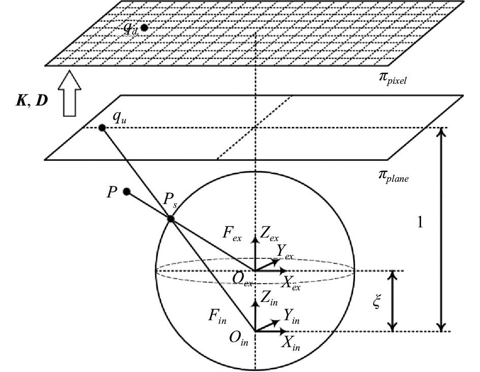
全方位相机模型与针孔相机的成像模型不同,其成像模型示意如图1所示[19]。

图 1 全方位相机成像模型
Figure 1. Omnidirectional camera imaging model
全方位相机主要有两个坐标系,分别是相机运动坐标系$ {F}_{ex} $和相机光学坐标系$ {F}_{in} $。如图1所示,两个坐标系并非完全重合,而是存在偏移量$ \xi $。它描述了镜头的非中心对称性,其物理含义可理解为相机光学坐标系的主点与光学中心之间的距离,单位为mm。
相机的成像过程可分为以下三步:1)世界点$ P $与光学中心$ {O}_{ex} $的连线交以$ {O}_{ex} $为球心的单位球于点$ {P}_{s} $;2)转换到坐标系$ {F}_{in} $中,$ {O}_{in} $与$ {P}_{s} $连线的延长线交相机成像平面$ {\pi }_{plane} $于点$ {q}_{u} $;3)$ {q}_{u} $与相机的内参矩阵$ \boldsymbol{K} $以及畸变系数矩阵$ \boldsymbol{D} $相计算,得到像素平面$ {\pi }_{pixel} $上最终成像点$ {q}_{d} $。文中实验所选用的全方位相机分辨率为4000 pixel×3000 pixel,其中CCD传感器尺寸为1/2.3 in(1 in=2.54 cm)。
-
文中采用两个棋盘格与二维码 (Checkerboard and Augmented Reality University of Cordoba,ChArUco)标定板进行标定。ChArUco标定板由传统棋盘格结合ArUco标记构成,如图2(a)所示。每个ArUco标记及标志点均有其特定可识别ID,且ArUco标记严格按照所规定的图案规则生成,顺序排列。ChArUco标定板允许相机在只找到标定板上部分区域时,也可获得相机与标定板之间的位姿关系。

图 2 相机与转轴标定。(a) ChArUco标定板;(b)标定系统示意图
Figure 2. Camera and axis calibration. (a) ChArUco calibration plate; (b) Schematic diagram of calibration system
常用解算标定板与相机位姿关系的方法为PnP(Perspective-n-Point)算法[20],其利用n对已知的三维世界点—二维像素点对建立二者之间的对应关系。如图2(b)所示,该方法中将两个标定板邻近摆放,相机多次旋转拍摄标定板;对两个标定板分别提取标志点,并计算两个世界坐标系到相机坐标系的变换矩阵$ {\boldsymbol{K}}_{{c}{h}1} $、$ {\boldsymbol{K}}_{{c}{h}2} $。
此时:
$$ \begin{array}{c}{\boldsymbol{c}}_{cam}={\boldsymbol{K}}_{{c}{h}1}{{{\boldsymbol{c}}}}_{w1}\text={\boldsymbol{K}}_{{c}{h}2}{{{\boldsymbol{c}}}}_{w2}\end{array} $$ (1) 式中:${{\boldsymbol{c}}_{cam} = \left[{x}_{cam},{y}_{cam},{z}_{cam}\right]}^{{\rm{T}}}$、${{\boldsymbol{c}}_{w1} = \left[{x}_{w1},{y}_{w1},{z}_{w1}\right]}^{{\rm{T}}}$、${{{\boldsymbol{c}}}}_{w2} = [{x}_{w2}, {y}_{w2},{z}_{w2}]^{{\rm{T}}}$分别为相机坐标系、坐标系1以及坐标系2中一点的坐标。由此可得:
$$ \begin{array}{c}{\boldsymbol{c}}_{w1}\text={\boldsymbol{K}}_{{c}{h}1}^{-1}{\boldsymbol{K}}_{{c}{h}2}{\boldsymbol{c}}_{w2}\stackrel{\scriptscriptstyle\mathrm{def}}={\boldsymbol{K}}_{{c}{h}}{\boldsymbol{c}}_{w2}\end{array} $$ (2) 式中:$ {\boldsymbol{K}}_{{c}{h}}={\boldsymbol{K}}_{{c}{h}1}^{-1}{\boldsymbol{K}}_{{c}{h}2} $为世界坐标系2到坐标系1的变换矩阵。
-
文中所提基于全方位相机-转轴标定方法的系统标定流程图如图3所示。

图 3 系统标定流程图
Figure 3. System calibration flow chart
主要分为以下步骤,首先根据全方位相机的模型计算相机内参;之后以固定角度为步长旋转拍摄特殊标定板;利用PnP算法解算相机坐标系与两个标定板(世界)坐标系之间的位姿关系;接下来由若干个相机光心坐标拟合出轴的位置,并解算光心在轴坐标系下的坐标;利用最小二乘法获得世界坐标系与轴坐标系之间的位姿,结合PnP结果得到相机与转轴之间的位姿初值;最后对上述求得的初值进行优化,获得准确位姿。
-
两世界坐标系外参可根据1.2节求得。为方便计算,后续所有坐标系2中的坐标数据将根据$ {\boldsymbol{K}}_{{c}{h}} $转换到坐标系1中,下文中世界坐标系即为坐标系1。
假设采集完成后,两个标定板共有可用于计算位姿的位置n个。分别对每个位置拍摄的标定板图片进行提取标志点操作,求得第i相机坐标系到世界坐标系1或世界坐标系2的变换矩阵,并完成变换矩阵从坐标系2到坐标系1的转换,最终位姿为$ {\boldsymbol{K}}_{{i}\left|{n}\right.} $,于是便可得到:
$$ \begin{array}{c}{\boldsymbol{c}}_{{i}\left|{w}\right.}={\boldsymbol{K}}_{{i}\left|{n}\right.}{\boldsymbol{c}}_{{i}\left|{c}\right.}\text{,}i=\mathrm{1,2},3,\cdots ,n\end{array} $$ (3) 式中:${\boldsymbol{c}}_{{i}\left|{c}\right.}={\left[{x}_{i\left|c\right.},{y}_{i\left|c\right.},{z}_{i\left|c\right.}\right]}^{{\rm{T}}}$为第i个位置相机坐标系中的点;${{\boldsymbol{c}}_{{i}\left|{w}\right.}=\left[{x}_{i\left|w\right.},{y}_{i\left|w\right.},{z}_{i\left|w\right.}\right]}^{{\rm{T}}}$为该点对应的世界坐标系点坐标。
令${\boldsymbol{c}}_{{i}\left|{c}\right.}={\left[\mathrm{0,0},0\right]}^{{\rm{T}}}$,代入公式(3)中便可以得到第i个位置处相机光心的世界坐标,设其为${{{\boldsymbol{c}}}}_{i}=[{x}_{i\left|O\right.}, {y}_{i\left|O\right.},{z}_{i\left|O\right.}]^{{\rm{T}}}$。
-
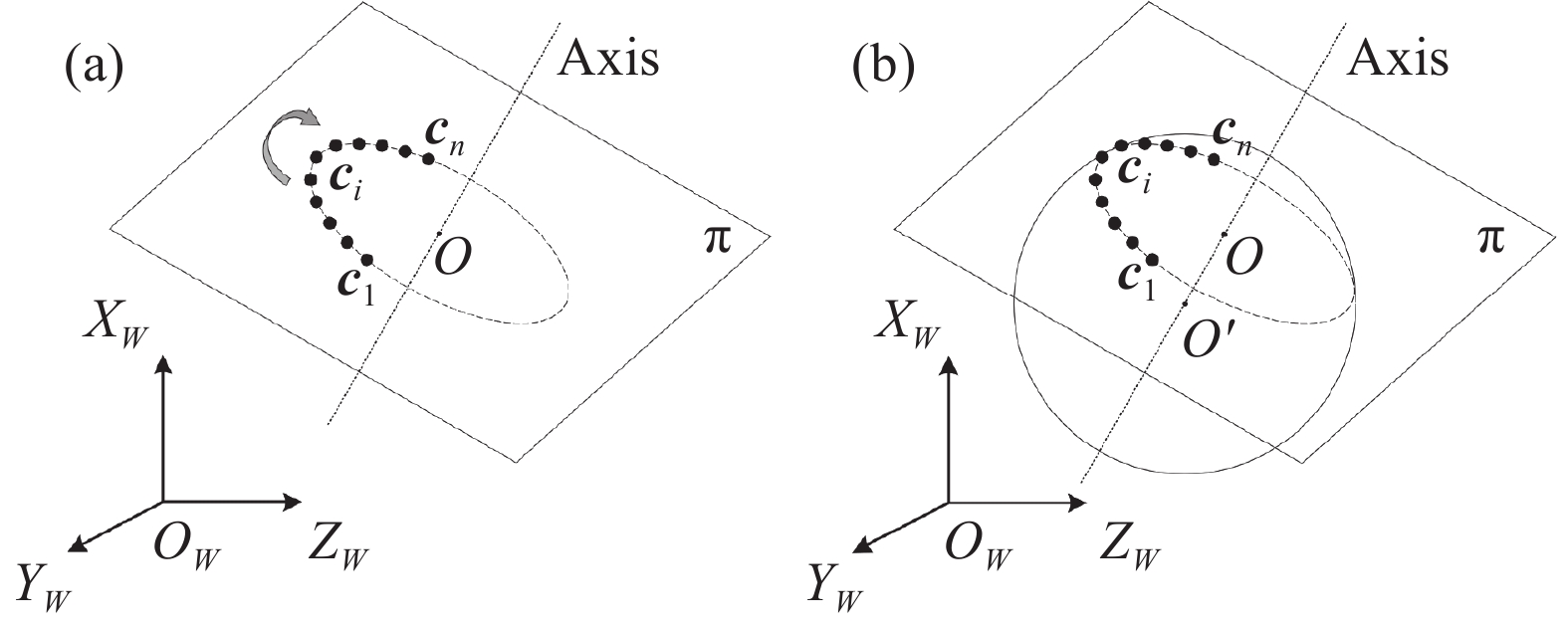
在相机拍摄过程当中,若选择世界坐标系为参考坐标系,此时相机可视为在空间中绕转轴做圆周运动。实际上,由于转轴在旋转过程中的机械振动,转轴装配误差等因素,光心存在位于旋转平面上下的细小偏差。如图4(a)所示, n个光心由$ {{\boldsymbol{c}}}_{1} $~$ {{\boldsymbol{c}}}_{n} $顺序排列,设光心所在平面为$ \mathrm{\pi } $,转轴所在直线为Axis,转轴与旋转平面交点为点$ O $。

图 4 光心轨迹拟合。(a)光心平面拟合;(b)光心球面拟合
Figure 4. Trajectory fitting of optical center. (a) Plane fitting of optical center; (b) Spherical fitting of optical center
根据已知光心点坐标,利用非线性最小二乘法对平面进行拟合。非线性最小二乘法通过求解目标函数的雅可比矩阵,找到目标函数减小最快的参数变化方向,迭代调整参数值使目标函数达到最小。最小二乘法中常用算法主要有Levenberg-Marquardt法[21],以及高斯-牛顿法[22],文中最小二乘算法基于L-M算法。针对此节拟合平面,预设平面$ \mathrm{\pi } $的表达式为$ ax+by+cz+d=0 $,则其代价方程的最小二乘形式可表达为:
$$ \begin{array}{c}\underset{{a}^{\mathrm{*}},{b}^{\mathrm{*}},{c}^{\mathrm{*}}}{\mathrm{min}}\dfrac{1}{2}\displaystyle\sum _{i=1}^{n}{\| d-\left({{a}^{\mathrm{*}}x}_{i\left|O\right.}+{b}^{\mathrm{*}}{y}_{i\left|O\right.}+{c}^{\mathrm{*}}{z}_{i\left|O\right.}\right)\|}^{2}\end{array} $$ (4) 根据球的性质,当空间中一球被平面所截时,球心到截面的垂线交截圆于截圆圆心,即球心与截圆圆心连线方向为平面法线方向。对光心点进行球面拟合,球心为$ {O}{{{'}}} $,球$ {O}{{{'}}} $被平面$ \mathrm{\pi } $所截圆可视为光心运动轨迹,如图4(b)所示。球面拟合代价方程为:
$$\begin{split} {{\boldsymbol{O}}{{{'}}}}^{\mathrm{*}}=& \underset{{x}_{0}^{\mathrm{*}},{y}_{0}^{\mathrm{*}},{z}_{0}^{\mathrm{*}}}{\mathrm{min}}\dfrac{1}{2}\displaystyle\sum _{i=1}^{n}\|{r}^{2}-\left[{\left({x}_{i\left|O\right.}-{x}_{0}^{\mathrm{*}}\right)}^{2}+\left({y}_{i\left|O\right.}-{y}_{0}^{\mathrm{*}}\right)^{2}+\right.\\ &\left.{ \left({z}_{i\left|O\right.}-{z}_{0}^{\mathrm{*}}\right)}^{2}\right]\|^{2} \end{split} $$ (5) 式中:${{{\boldsymbol{O}}{{{'}}}}^{\mathrm{*}}=\left[{x}_{0}^{\mathrm{*}},{y}_{0}^{\mathrm{*}},{z}_{0}^{\mathrm{*}}\right]}^{{\rm{T}}}$为待拟合的球心坐标;$ r $为待拟合球的半径。
已知平面$ \mathrm{\pi } $法向量为${\left[{a}^{\mathrm{*}},{b}^{\mathrm{*}},{c}^{\mathrm{*}}\right]}^{{\rm{T}}}$,球心坐标为${{\boldsymbol{O}}{{{'}}}}^{\mathrm{*}}={\left[{x}_{0}^{\mathrm{*}},{y}_{0}^{\mathrm{*}},{z}_{0}^{\mathrm{*}}\right]}^{{\rm{T}}}$,根据直线点法式,可得转轴所在直线方程为:
$$ \begin{array}{c}\dfrac{x-{x}_{0}^{\mathrm{*}}}{{a}^{\mathrm{*}}}=\dfrac{y-{y}_{0}^{\mathrm{*}}}{{b}^{\mathrm{*}}}=\dfrac{z-{z}_{0}^{\mathrm{*}}}{{c}^{\mathrm{*}}}\end{array} $$ (6) -
将转轴所在直线方程与平面$ \mathrm{\pi } $表达式联立:
$$ \begin{array}{c}\left\{\begin{array}{c}{a}^{\mathrm{*}}{x}_{axis}+{b}^{\mathrm{*}}{y}_{axis}+{c}^{\mathrm{*}}{z}_{axis}+d=0\\ \dfrac{{x}_{axis}-{x}_{0}^{\mathrm{*}}}{{a}^{\mathrm{*}}}=\dfrac{{y}_{axis}-{y}_{0}^{\mathrm{*}}}{{b}^{\mathrm{*}}}=\dfrac{{z}_{axis}-{z}_{0}^{\mathrm{*}}}{{c}^{\mathrm{*}}}\end{array}\right.\end{array} $$ (7) 解方程组即可获得交点$ O $的世界坐标$[{x}_{axis}, {y}_{axis},{z}_{axis}]^{{\rm{T}} }$。
设第一个相机光心$ {{\boldsymbol{c}}}_{1} $在平面$ \mathrm{\pi } $上的投影点为$ {{\boldsymbol{c}}}_{1}{{{'}}} $。以点$ O $为原点建立轴坐标系,指定沿平面法向量向上为轴坐标系$ Z $轴方向,由$ O $点指向投影点$ {{\boldsymbol{c}}}_{1}{{{'}}} $方向为$ Y $轴,则$ X $轴方向向量可以由$ Y $、$ Z $轴方向向量叉积求得。所建轴坐标系如图5所示。

图 5 轴坐标系的建立
Figure 5. Establishment of axis coordinate system
各个光心点在轴坐标系下的坐标${\boldsymbol{c}}_{i}=[{x}_{i\left|a\right.}, {y}_{i\left|a\right.},{z}_{i\left|a\right.}]^{{\rm{T}}}$,可根据向量$\overrightarrow{{{\boldsymbol{c}}}_{1}{{{'}}}{{\boldsymbol{c}}}_{{i}}}$在$ {X}_{A} $、$ {Y}_{A} $、$ {Z}_{A} $轴正方向上的投影给出:
$$ \begin{array}{c}{\boldsymbol{c}}_{i}=\left|\overrightarrow{{{\boldsymbol{c}}}_{1}{{{'}}}{{\boldsymbol{c}}}_{{i}}}\right|\left[\begin{array}{c}\mathrm{cos}{\theta }_{x}\\ 1+\mathrm{cos}{\theta }_{y}\\ \mathrm{cos}{\theta }_{z}\end{array}\right]\end{array} $$ (8) 式中:$ {\theta }_{x} $、$ {\theta }_{y} $、$ {\theta }_{z} $分别为向量$\overrightarrow{{{\boldsymbol{c}}}_{1}{{{'}}}{{\boldsymbol{c}}}_{{i}}}$与$ {X}_{A} $、$ {Y}_{A} $、$ {Z}_{A} $轴正方向的夹角,其余弦值如公式(9)所示:
$$\begin{split} &{\left[\begin{array}{ccc}\mathrm{cos}{\theta }_{x}& \mathrm{cos}{\theta }_{y}& \mathrm{cos}{\theta }_{z}\end{array}\right]}^{{\rm{T}}}= \left[\begin{array}{ccc}\overrightarrow{{\boldsymbol{e}}_{{x}}}& 0& 0\\ 0& \overrightarrow{{\boldsymbol{e}}_{{y}}}& 0\\ 0& 0& \overrightarrow{{\boldsymbol{e}}_{{z}}}\end{array}\right]\times\\ & {\left[\begin{array}{ccc}\dfrac{\overrightarrow{{\boldsymbol{c}}_{1}{'}{\boldsymbol{c}}_{i}}}{\left|\overrightarrow{{\boldsymbol{c}}_{1}{'}{\boldsymbol{c}}_{i}}\right|}& \dfrac{\overrightarrow{{\boldsymbol{c}}_{1}{'}{\boldsymbol{c}}_{i}}}{\left|\overrightarrow{{\boldsymbol{c}}_{1}{'}{\boldsymbol{c}}_{i}}\right|}& \dfrac{\overrightarrow{{\boldsymbol{c}}_{1}{'}{\boldsymbol{c}}_{i}}}{\left|\overrightarrow{{\boldsymbol{c}}_{1}{'}{\boldsymbol{c}}_{i}}\right|}\end{array}\right]}^{{\rm{T}}} \end{split} $$ (9) 式中:$ \overrightarrow{{\boldsymbol{e}}_{{x}}} $、$ \overrightarrow{{\boldsymbol{e}}_{{y}}} $、$ \overrightarrow{{\boldsymbol{e}}_{{z}}} $分别为$ {X}_{A}\mathrm{、}{Y}_{A}\mathrm{、}{Z}_{A} $轴的单位方向向量。
根据公式(3)、(8),n个光心点的世界坐标和轴坐标均已求得。将坐标转换为XYZ格式的点云数据,并基于ICP(Iterative Closest Point)算法[23]计算两组坐标值之间的变换矩阵初值。之后利用初值,根据非线性最小二乘原理对世界-转轴坐标系之间的变换矩阵$ {\boldsymbol{K}}_{{A}2{W}} $进行优化计算。此时可得:
$$ \begin{array}{c}{\boldsymbol{c}}_{{W}}={\boldsymbol{K}}_{{A}2{W}}{\boldsymbol{c}}_{{A}}\end{array} $$ (10) 式中:$ {\boldsymbol{c}}_{{A}} $为轴坐标系中的坐标;$ {\boldsymbol{c}}_{{W}} $为世界坐标系中的坐标。由公式(3)可得第i个相机坐标系与世界坐标系之间的变换矩阵$ {\boldsymbol{K}}_{{i}\left|{n}\right.} $。由于设定轴坐标系的$ {Y}_{A} $轴穿过首个相机位置光心,故以第一个相机位置为参考进行计算:
$$ \begin{array}{c}{\boldsymbol{c}}_{{W}}={\boldsymbol{K}}_{1\left|{n}\right.}{\boldsymbol{c}}_{1\left|{C}\right.}={\boldsymbol{K}}_{{A}2{W}}{\boldsymbol{c}}_{{A}}\end{array} $$ (11) 式中:$ {\boldsymbol{c}}_{1\left|{C}\right.} $为第一个位置相机坐标系中的坐标。于是:
$$ \begin{array}{c}{\boldsymbol{c}}_{{A}}={{\boldsymbol{K}}_{{A}2{W}}^{-1}\boldsymbol{K}}_{1\left|{n}\right.}{\boldsymbol{c}}_{1\left|{C}\right.}\stackrel{\scriptscriptstyle\mathrm{def}}={\boldsymbol{K}}_{{C}2{A}}{{{\boldsymbol{c}}}}_{1\left|{C}\right.}\end{array} $$ (12) 最终,相机与转轴之间的变换矩阵${\boldsymbol{K}}_{{C}2{A}}={{\boldsymbol{K}}_{{A}2{W}}^{-1}{K}}_{1\left|{n}\right.}$即为所求。
-
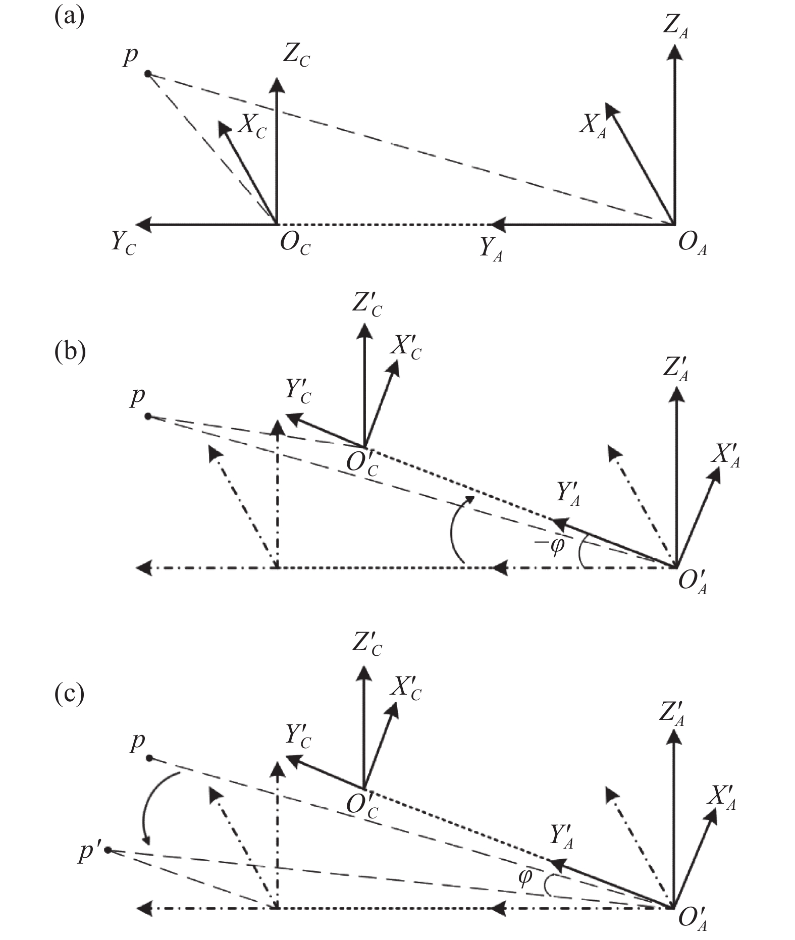
公式(12)中,变换矩阵是基于解析几何得出,需对其进行优化,获得准确位姿。以${\boldsymbol{K}}_{{C}2{A}}$为初值进行迭代,可有效防止优化问题陷入局部最优解中。BA算法是一种用于优化相机姿态和三维点位置的优化算法。通过最小化重投影误差,将观测到的特征点和相机的姿态进行联合优化。重投影误差优化模型如图6所示,计算被分为五个部分。

图 6 相机-转轴重投影模型。(a)原始模型;(b)旋转后模型;(c)等效模型
Figure 6. Camera-axis reprojection model. (a) Original model; (b) After-rotation model; (c) Equivalent model
1)设相机旋转至第i个位置,拍摄到特征点$ p $,但此时暂且令相机与转轴依然在初始位置,见图6(a)。首先将点$ p $世界坐标$ {\boldsymbol{p}}_{{W}} $转换至第一个相机坐标系中,再利用公式(12)中的变换矩阵初值,获得点$ p $的轴坐标系坐标$ {\boldsymbol{p}}_{{A}} $,其表达式为:
$$ \begin{array}{c}{\boldsymbol{p}}_{{A}}={\boldsymbol{K}}_{{C}2{A}}{\boldsymbol{p}}_{{C}}={\boldsymbol{K}}_{{C}2{A}}{\boldsymbol{K}}_{1\left|{n}\right.}^{-1}{\boldsymbol{p}}_{{W}}\end{array} $$ (13) 2)转轴与相机顺时针旋转$ \varphi $至第i个位置,如图6(b)所示,此时拍摄到点$ p $;
3)根据相对运动,若以相机为参考系,可看作点$ p $绕转轴逆时针旋转$ \varphi $至点$ {p}{{{'}}} $,如图6(c)所示。根据三维点的旋转坐标变换,可得变换之后的轴坐标系坐标$ {\boldsymbol{p}}_{{A}}' $为:
$$ \begin{array}{c}{\boldsymbol{p}}_{{A}}{'}={\boldsymbol{T}}{\boldsymbol{p}}_{{A}}=\left[\begin{array}{ccc}\mathrm{cos}\varphi & -\mathrm{sin}\varphi & 0\\ \mathrm{sin}\varphi & \mathrm{cos}\varphi & 0\\ 0& 0& 1\end{array}\right]{\boldsymbol{p}}_{{A}}\end{array} $$ (14) 4)将所得点坐标${\boldsymbol{p}}_{{A}}{{{'}}}$投影至相机图像平面中,与实际拍摄到的点$ p $建立代价方程,对位姿进行联合迭代优化:
$$ \begin{array}{c}\left({\boldsymbol{\varPhi }}^{\mathrm{*}},{\boldsymbol{t}}^{\mathrm{*}}\right)=\underset{{\boldsymbol{\varPhi }}^{\mathrm{*}},{\boldsymbol{t}}^{\mathrm{*}}}{{\min}}\dfrac{1}{2}\displaystyle\sum _{i=1}^{n}{\| \boldsymbol{u}-\boldsymbol{K}\boldsymbol{D}{{\boldsymbol{K}}_{{C}2{A}}^{-1}\boldsymbol{p}}_{{A}}{{{'}}}\|}^{2}\end{array} $$ (15) 式中:$\boldsymbol{\varPhi }$为代表相机到轴旋转李群$ \boldsymbol{R} $的李代数形式;$ \boldsymbol{t} $为相机到轴平移向量;$ \boldsymbol{u} $为该标志点在图像中的像素坐标;$ \boldsymbol{K} $为相机内参矩阵;$ \boldsymbol{D} $为畸变系数矩阵。
5)经过优化之后,${\boldsymbol{\varPhi }}^{\mathrm{*}}$经Rodrigues公式变换可得到旋转矩阵$ {\boldsymbol{R}}^{\mathrm{*}} $,最终与平移向量$ {\boldsymbol{t}}^{\mathrm{*}} $一起构成变换矩阵$ {\boldsymbol{K}}_{{C}2{A}}^{\mathrm{*}}=\left[\begin{array}{cc}{\boldsymbol{R}}^{\mathrm{*}}& {\boldsymbol{t}}^{\mathrm{*}}\end{array}\right] $。
-
基于全方位相机的转轴旋转标定系统主要由一个全方位彩色相机、一个转台、两个ChArUco标定板组成,实验系统的整体结构如图7所示。其中全方位相机型号为MJ7039 A-SPEC01-01,分辨率为4000 pixel×3000 pixel,CCD传感器尺寸为1/2.3 in,有效焦距为3.3 mm;转台型号为:720云-LG-01,其角分辨率为1°;两个ChArUco标定板均采用9×12规格,棋盘格大小为45 mm×45 mm,ArUco结构码采用OpenCV库中的DICT_6 X6_250规则进行编码。

图 7 基于全方位相机的转轴标定系统
Figure 7. Axis calibration system based on omnidirectional camera
-
根据1.1节中所介绍模型,对全方位相机内参进行标定。利用张正友标定法获得等效焦距$ {f}_{x} $、$ {f}_{y} $,以及主点坐标$ {c}_{x} $、$ {c}_{y} $,并通过OpenCV库单独对偏移量$ \xi $进行标定。内参标定结果如表1所示。
表 1 相机内参及偏移量
Table 1. Camera internal parameters and offset
Focal distance/pixel Principal point/pixel $ \xi $/mm $ {f}_{x} $ $ {f}_{y} $ $ {c}_{x} $ $ {c}_{y} $ 4344.8 4347.8 2025.9 1467.0 0.9521 标定重投影误差及相机畸变系数如表2所示。其中Mean-RE (Mean-Reprojection Error)为平均重投影误差,Max-RE (Maximum-Reprojection Error)为最大重投影误差,$ {k}_{1} $、$ {k}_{2} $为径向畸变系数,$ {p}_{1} $、$ {p}_{2} $为切向畸变系数。
表 2 相机的重投影误差及畸变系数
Table 2. Reprojection error and distortion coefficient of camera
Projection error/pixel ${k}_{_1}$ ${k}_{_2}$ ${p}_{_1}$ ${p}_{_2}$ Mean-RE Max-RE 0.1276 0.2422 −0.5539 0.2754 −0.00046 −0.00103 -
该实验转轴每次旋转为固定角度3°,转轴共转动180°,转动60次。当图片采集到的标志点数小于预定义阈值时,认为使用其计算位姿不可靠,该图片将不参与计算。对每个位置使用PnP算法之后,可得到相机坐标系与世界坐标系之间的变换矩阵$ {\boldsymbol{K}}_{{C}2{W}} $,并计算得光心在空间中的分布。利用Ceres库对平面进行拟合,拟合平面的表达式为:
$$ \begin{array}{c}2.166x-0.020\;3y+z-588.4=0\end{array} $$ (16) 所求得光心及拟合平面如图8(a)所示。

图 8 拟合及处理。(a)平面拟合;(b)球面拟合;(c)建立轴坐标系
Figure 8. Fitting and processing. (a) Plane fitting; (b) Spherical fitting; (c) Establish axis coordinate system
继续由光心点拟合球,如图8(b)所示,球心坐标为${\left[\mathrm{82.090\;4,253.086\;4,253.622\;2}\right]}^{{\rm{T}}}$,半径为100 mm。
按照2.4小节中所述方法,建立轴坐标系$ {{O}}_{{a}}- {{X}}_{{a}}{{Y}}_{{a}}{{Z}}_{{a}} $,如图8(c)所示。
同时,根据拟合结果,计算所拟合平面的平面度误差以及拟合旋转轨迹的圆度误差,其中圆度拟合标准差为0.0218 mm,平面度拟合标准差为0.0301 mm。
-
通过所建轴坐标系,根据公式(8)可得到光心点在轴坐标系下的坐标。根据两组坐标值,利用传统ICP算法求得两组坐标之间的位姿;之后将ICP的结果作为初值,利用Ceres库对两组坐标值做最小二乘优化,可得到由轴坐标系到世界坐标系的变换矩阵$ {\boldsymbol{K}}_{{A}2{W}} $。ICP计算以及优化之后的位姿结果如表3所示。
表 3 两种方法计算位姿结果
Table 3. Two methods to calculate posture results
Method Rotation matrix R Translation vector T ICP $\left[\begin{array}{ccc}0.285\;8 & 0.306\;0& 0.908\;1\\ -0.717\;7& 0.696\;3& -0.008\;8\\ -0.635\;0& -0.649\;2& 0.418\;6\end{array}\right]$ $ \left[\begin{array}{c}144.062\\ 251.727\\ 281.533\end{array}\right] $ Optimization of Ceres library $\left[\begin{array}{ccc}0.338\;2& 0.247\;7& 0.907\;8\\ -0.575\;8& 0.817\;6& -0.008\;5\\ -0.744\;4& -0.519\;9& 0.419\;1\end{array}\right]$ $ \left[\begin{array}{c}143.765\\ 252.508\\ 282.094\end{array}\right] $ 根据变换矩阵$ {\boldsymbol{K}}_{{C}2{W}} $,可初步计算得相机与转轴之间的位姿${\boldsymbol{K}}_{{C}2{A}}$。三个坐标系之间,两两变换矩阵对应的旋转向量与平移向量如表4所示。
表 4 旋转向量与平移向量
Table 4. Rotation vector and translation vector
Correspondence Rotation vector ${\boldsymbol{\varPhi }} $ Translation vector $ {{\boldsymbol{t}}} $ Camera-world ${\left[0.543, -2.734, -1.315\right]}^{{\rm{T}}}$ ${\left[290.792, -306.674, -69.305\right]}^{{\rm{T}}}$ Axis-world ${\left[-0.341, 1.103, -0.550\right]}^{{\rm{T}}}$ ${\left[143.765, 252.508, 282.094\right]}^{{\rm{T}}}$ Camera-axis ${\left[-\mathrm{1.477,1.475}, 1.014\right]}^{{\rm{T}}}$ ${\left[-3.025\times {10}^{-5},73.445, -0.0017\right]}^{{\rm{T}}}$ 将${\boldsymbol{K}}_{{C}2{A}}$对应的旋转向量$ \boldsymbol{\varPhi } $以及平移向量$ \boldsymbol{t} $作为初值,对相机与转轴之间的位姿进行迭代优化。
根据文中所提方法,最终得到位姿$ {\boldsymbol{\varPhi }}^{\mathrm{*}} $、$ {\boldsymbol{t}}^{\mathrm{*}} $的优化值分别为${\left[-1.475, 1.474, 1.015\right]}^{{\rm{T}}}$和$[0.027, 73.299, -0.002]^{{\rm{T}}}$。
利用优化结果,计算经过优化后每个光心点到转轴的距离与转轴转角之间的关系,计算结果如图9所示。其中距离的极差为0.085 mm,标准差为0.021 mm,符合标定精度的测量要求。

图 9 不同角度光心到转轴的距离
Figure 9. Distance from optical center to axis at different angles
为定性验证相机与转轴外参标定结果的精度,使用实验系统对室外环境进行多次旋转拍摄,每两次拍摄之间夹角为60°,并根据所求外参,将多次拍摄的单个图像拼接为一张全景图像,拼接效果如图10所示。
继续检验文中系统鲁棒性,分别改变相机与转轴之间的半径,以及相机与两个标定板之间的距离,进行多次实验,各组光心的世界坐标如图11所示。

图 10 单张图片与全景图片拼接结果
Figure 10. The stitching results of single images and panoramic images

图 11 三组实验条件下的光心点分布
Figure 11. The distribution of optical center points under three experimental conditions
分别对三组实验数据当中对应的旋转向量与平移向量进行求解,求得三组位姿如表5所示,两两之间位姿差异较小。
表 5 三组实验条件下的位姿
Table 5. Pose under three groups of experimental conditions
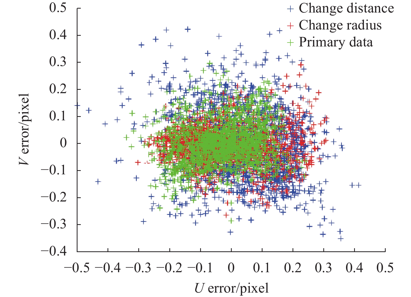
Condition Rotation vector $ {\boldsymbol{\varPhi }} $ Translation vector $ {{\boldsymbol{t}}} $ Primary data ${\left[-1.475, 1.474, 1.015\right]}^{{\rm{T}}}$ ${\left[0.027, 73.299, -0.002\right]}^{{\rm{T}}}$ Change distance ${\left[-1.473, 1.485, 1.004\right]}^{{\rm{T}}}$ ${\left[-0.001, 73.408, -0.003\right]}^{{\rm{T}}}$ Change radius ${\left[-\mathrm{1.472,1.479}, 1.006\right]}^{{\rm{T}}}$ ${\left[-1.831\times {10}^{-4}, 73.315, -0.002\right]}^{{\rm{T}}}$ 根据表5中所求三组位姿,分别计算各组的重投影误差,并绘制出重投影点,最终结果如图12所示。由其可看出参考组与半径变化组重投影相对集中于中间区域,距离变化组分布略为分散,但仍在合理范围内。

图 12 三组实验条件下的重投影误差分布
Figure 12. Error distribution of reprojection under three groups of experimental conditions
同时,为进一步定量分析系统精度,分别绘制每组中两个方向重投影误差分布直方图,如图13所示。

图 13 重投影误差直方图。(a)参考组U方向;(b)参考组V方向;(c)半径变化组U方向;(d)半径变化组V方向;(e)距离变化组U方向;(f)距离变化组V方向
Figure 13. Projection error histogram. (a) U direction of reference group; (b) V direction of reference group; (c) U direction of radius change group; (d) V direction of radius change group; (e) U direction of distance change group; (f) V direction of distance change group
其中参考组两个方向平均重投影误差BMPE分别为0.116 7 pixel和0.095 4 pixel,半径变化组为0.103 9 pixel和0.080 2 pixel,距离变化组中投影点相对较为分散,但95%以上均落在$ \left[-0.25,\mathrm{ }0.25\right] $区间内,且两个方向的BMPE分别为0.141 6 pixel和0.127 6 pixel。且如图10所示,利用旋转拍摄单张图像合成全景图像效果良好,拼接处平滑过渡,进一步验证了文中方法的准确性。
-
针对相机与转轴之间位姿不确定的问题,文中提出了一种基于全方位相机和双ChArUco标定板的标定方法。通过建立坐标系变换的数学模型,计算并优化相机与转轴之间的位姿关系,有效抑制了随机误差对实验的影响。实验结果证明该方法可实现相机与转轴之间的距离精度达到亚毫米级,经过优化后的平均重投影误差可控制在0.15 pixel以下。相较于其他方法,文中所提方法系统复杂度低,使用两个标定板进行标定提高了系统的精度,且有效避免了因摆放位置带来的随机误差。系统仅需利用相机对固定位置的两个特殊标定板进行旋转拍摄,本身系统复杂程度不高,易于实现,能可靠地应用于不同场景的拍摄工作,且对轴坐标系的定义比较灵活,系统鲁棒性高,实验精度均在可靠范围之内,该方法的有效性得到了验证。
Research on pose calibration method for omnidirectional camera and rotation axis
-
摘要: 在利用相机对物体进行感知的过程中,标定相机与外界参考系之间的位姿是测量中至关重要的一环,能否精准确定二者之间的外参决定着最终三维信息质量的好坏。然而在传统的测量系统当中,测量物体尺寸受限于针孔相机视场的大小。相比较而言,全方位相机具有视场广、成像质量高等优点,常配合旋转系统进行全景图像生成,也可配合激光雷达点云生成场景全景模型,为目前大场景测量的主流方向。就目前存在于相机与旋转系统之间外参标定的复杂问题,文中提出了一种针对全方位相机与旋转轴之间的标定方法。该方法通过使用全方位相机,对两个二维码棋盘格进行旋转拍摄,同时通过理论推导建立起可靠的数学模型作为原理支撑,并利用光束法平差,对基于解析法获得的初步结果进行再次优化,从而获得更精确的外参估计。该方法对设备安装精度要求不高,只需在相机视场范围内,考虑标定板与全方位相机之间的摆放位置即可。实验结果表明,该方法经过优化后的平均重投影误差可控制在0.15 pixel以下,满足实验测量要求,并在不同场景下展现了良好的应用效果。Abstract:
Objective Accurate determination of camera-to-reference frame parameters is crucial. Traditional systems are limited by camera field of view, constraining object size measurability. Omnidirectional cameras offer wide view and high imaging quality by using rotation systems or combining with LiDAR for scene modeling. This paper proposes a calibration method for omnidirectional camera and rotation axis. It uses omnidirectional cameras to capture rotation of QR code chessboards. A reliable mathematical model and nonlinear fitting optimize initial results for accurate parameter estimation. This method has low equipment requirements, considering board placement within the camera's view. The experimental results indicate that the average optimized reprojection error of this method can be controlled below 0.15 pixel, satisfying the requirements of experimental measurements and demonstrating promising application performance in various scenarios. Methods A reliable system is proposed to calibrate the extrinsic parameters between the camera and the rotation axis. A omnidirectional camera with a resolution of 4 000 pixel×3 000 pixel is utilized to capture the dual ChArUco calibration boards (Fig.2). For the extrinsic calibration, an algorithm is designed to fit the rotation plane and different methods for establishing the axis coordinate system are introduced (Fig.5). The accuracy of the system is evaluated using the distance from the optical center to the origin of the axis coordinate system (Fig.9) and the reprojection errors under different conditions (Fig.11). Results and Discussions In this method, the Perspective-n-Point algorithm is employed to determine the camera's optical center coordinates. Subsequently, a nonlinear least squares fitting technique is applied to fit the rotation plane and sphere of the optical center (Fig.8). The circularity fitting standard deviation for the intersection between the plane and the sphere is measured to be 0.021 8 mm, while the flatness fitting standard deviation is 0.030 1 mm. The range of distances from the camera's optical center to the axis is found to be 0.085 mm, with a standard deviation of 0.021 mm (Fig.9). Additionally, the maximum reprojection error between the experimental reference group and the other two control groups is 0.141 6 pixel (Fig.12), thereby validating the accuracy of the proposed method. Conclusions To address the issue of pose uncertainty between the camera and the rotation axis, this paper proposes a calibration method based on a omnidirectional camera and dual ChArUco calibration boards. The method captures multiple sets of images containing the dual targets to obtain the position information of the camera's optical center at each shooting position. By establishing a mathematical model for coordinate system transformation, the pose relationship between the camera and the rotation axis is computed and optimized, effectively suppressing the influence of random errors in the experiments. Experimental results demonstrate that the proposed method achieves sub-millimeter-level accuracy in the distance between the camera and the rotation axis, with an average optimized reprojection error controlled below 0.15 pixel. Compared to other methods, the method presented in this paper has lower system complexity, improved accuracy by use of two calibration boards, and effectively mitigates random errors caused by placement variations. The results indicate that this method exhibits good robustness and convenience, making it reliably applicable to shooting tasks in diverse scenarios. -
Key words:
- optical measurement /
- omnidirectional camera /
- rotation axis /
- pose calibration /
- panoramic survey
-
图 2 相机与转轴标定。(a) ChArUco标定板;(b)标定系统示意图
Figure 2. Camera and axis calibration. (a) ChArUco calibration plate; (b) Schematic diagram of calibration system
图 4 光心轨迹拟合。(a)光心平面拟合;(b)光心球面拟合
Figure 4. Trajectory fitting of optical center. (a) Plane fitting of optical center; (b) Spherical fitting of optical center
图 6 相机-转轴重投影模型。(a)原始模型;(b)旋转后模型;(c)等效模型
Figure 6. Camera-axis reprojection model. (a) Original model; (b) After-rotation model; (c) Equivalent model
图 8 拟合及处理。(a)平面拟合;(b)球面拟合;(c)建立轴坐标系
Figure 8. Fitting and processing. (a) Plane fitting; (b) Spherical fitting; (c) Establish axis coordinate system
图 10 单张图片与全景图片拼接结果
Figure 10. The stitching results of single images and panoramic images
图 11 三组实验条件下的光心点分布
Figure 11. The distribution of optical center points under three experimental conditions
图 12 三组实验条件下的重投影误差分布
Figure 12. Error distribution of reprojection under three groups of experimental conditions
图 13 重投影误差直方图。(a)参考组U方向;(b)参考组V方向;(c)半径变化组U方向;(d)半径变化组V方向;(e)距离变化组U方向;(f)距离变化组V方向
Figure 13. Projection error histogram. (a) U direction of reference group; (b) V direction of reference group; (c) U direction of radius change group; (d) V direction of radius change group; (e) U direction of distance change group; (f) V direction of distance change group
表 1 相机内参及偏移量
Table 1. Camera internal parameters and offset
Focal distance/pixel Principal point/pixel $ \xi $/mm $ {f}_{x} $ $ {f}_{y} $ $ {c}_{x} $ $ {c}_{y} $ 4344.8 4347.8 2025.9 1467.0 0.9521  下载: 导出CSV
表 2 相机的重投影误差及畸变系数
Table 2. Reprojection error and distortion coefficient of camera
Projection error/pixel ${k}_{_1}$ ${k}_{_2}$ ${p}_{_1}$ ${p}_{_2}$ Mean-RE Max-RE 0.1276 0.2422 −0.5539 0.2754 −0.00046 −0.00103
下载: 导出CSV
表 3 两种方法计算位姿结果
Table 3. Two methods to calculate posture results
Method Rotation matrix R Translation vector T ICP $\left[\begin{array}{ccc}0.285\;8 & 0.306\;0& 0.908\;1\\ -0.717\;7& 0.696\;3& -0.008\;8\\ -0.635\;0& -0.649\;2& 0.418\;6\end{array}\right]$ $ \left[\begin{array}{c}144.062\\ 251.727\\ 281.533\end{array}\right] $ Optimization of Ceres library $\left[\begin{array}{ccc}0.338\;2& 0.247\;7& 0.907\;8\\ -0.575\;8& 0.817\;6& -0.008\;5\\ -0.744\;4& -0.519\;9& 0.419\;1\end{array}\right]$ $ \left[\begin{array}{c}143.765\\ 252.508\\ 282.094\end{array}\right] $
下载: 导出CSV
表 4 旋转向量与平移向量
Table 4. Rotation vector and translation vector
Correspondence Rotation vector ${\boldsymbol{\varPhi }} $ Translation vector $ {{\boldsymbol{t}}} $ Camera-world ${\left[0.543, -2.734, -1.315\right]}^{{\rm{T}}}$ ${\left[290.792, -306.674, -69.305\right]}^{{\rm{T}}}$ Axis-world ${\left[-0.341, 1.103, -0.550\right]}^{{\rm{T}}}$ ${\left[143.765, 252.508, 282.094\right]}^{{\rm{T}}}$ Camera-axis ${\left[-\mathrm{1.477,1.475}, 1.014\right]}^{{\rm{T}}}$ ${\left[-3.025\times {10}^{-5},73.445, -0.0017\right]}^{{\rm{T}}}$
下载: 导出CSV
表 5 三组实验条件下的位姿
Table 5. Pose under three groups of experimental conditions
Condition Rotation vector $ {\boldsymbol{\varPhi }} $ Translation vector $ {{\boldsymbol{t}}} $ Primary data ${\left[-1.475, 1.474, 1.015\right]}^{{\rm{T}}}$ ${\left[0.027, 73.299, -0.002\right]}^{{\rm{T}}}$ Change distance ${\left[-1.473, 1.485, 1.004\right]}^{{\rm{T}}}$ ${\left[-0.001, 73.408, -0.003\right]}^{{\rm{T}}}$ Change radius ${\left[-\mathrm{1.472,1.479}, 1.006\right]}^{{\rm{T}}}$ ${\left[-1.831\times {10}^{-4}, 73.315, -0.002\right]}^{{\rm{T}}}$
下载: 导出CSV
-
[1] Wan G Y, Wang Y, Wang T, et al. Automatic registration for panoramic images and mobile lidar data based on phase hybrid geometry index features [J]. Remote Sensing, 2022, 14(19): 4783. doi: 10.3390/rs14194783 [2] Wang M Y, Liu R F, Yang J B, et al. Traffic sign three-dimensional reconstruction based on point clouds and panoramic images [J]. The Photogrammetric Record, 2022, 37(177): 87-110. doi: 10.1111/phor.12398 [3] Berganski C, Hoffmann A, Möller R. Tilt correction of panoramic images for a holistic visual homing method with planar-motion assumption [J]. Robotics, 2023, 12(1): 00020. doi: 10.3390/robotics12010020 [4] 蒋荣飞. 车载高性能全景影像拼接算法研究[D]. 成都: 电子科技大学, 2022. Jiang R F. Research on high performance panoramic video stitching algorithm in vehicle[D]. Chengdu: School of Electronic Science and Engineering, 2022. (in Chinese) [5] Karam S, Nex F, Chidura B T, et al. Microdrone-based indoor mapping with graph SLAM [J]. Drones, 2022, 6(11): 352. doi: 10.3390/drones6110352 [6] 张恒, 侯家豪, 刘艳丽. 基于动态区域剔除的RGB-D视觉SLAM算法[J]. 计算机应用研究, 2022, 39(03): 675-680. Zhang H, Hou J H, Liu Y L. RGB-D visual SLAM algorithm based on dynamic region elimination [J]. Application Research of Computers, 2022, 39(3): 675-680. (in Chinese) [7] Hütten N, Meyes R, Meisen T. Vision transformer in industrial visual inspection [J]. Applied Sciences, 2022, 12(23): 11981. doi: 10.3390/app122311981 [8] Shi H, Lei X K, Wan F. Spatial calibration method for master-slave camera based on panoramic image mosaic [J]. Optical Engineering, 2019, 58(4): 043105. [9] 魏泊岩, 田庆国, 葛宝臻. 基于彩色编码相移条纹的相机标定[J]. 光电工程, 2021, 48(01): 200118. Wei B Y, Tian G Q, Ge B Z. Camera calibration based on color-coded phase-shifted fringe [J]. Opto-Electronic Engineering, 2021, 48(1): 200118. (in Chinese) [10] 胡志新, 王涛. 改进遗传算法优化BP神经网络的双目相机标定[J]. 电光与控制, 2022, 29(01): 75-79. Hu Z X, Wang T. Binocular camera calibration based on BP neural network optimized by improved genetic algorithm [J]. Electronics Optics & Control, 2022, 29(1): 75-79. (in Chinese) [11] 陈文艺, 许洁, 杨辉. 利用双神经网络的相机标定方法[J]. 红外与激光工程, 2021, 50(11): 20210071. doi: 10.3788/IRLA20210071 Chen W Y, Xu J, Yang H. Camera calibration method based on double neural network [J]. Infrared and Laser Engineering, 2021, 50(11): 20210071. (in Chinese) doi: 10.3788/IRLA20210071 [12] 侯艳丽, 苏显渝, 陈文静. 旋转视觉测量系统相机光心与转轴距离的标定方法[J]. 光学学报, 2022, 42(21): 2112001. doi: 10.3788/AOS202242.2112001 Hou Y L, Su X Y, Chen W J. Calibration method of distance between optical center of camera and rotation axis in rotating vision measurement system [J]. Acta Optica Sinica, 2022, 42(21): 2112001. (in Chinese) doi: 10.3788/AOS202242.2112001 [13] Cai X Q, Zhong K J, Fu Y J, et al. Calibration method for the rotating axis in panoramic 3D shape measurement based on a turntable [J]. Measurement Science and Technology, 2021, 32(3): 035004. doi: 10.1088/1361-6501/abcb7e [14] Livio B, Ramtin M, Matteo P, et al. Automatic calibration of a two-axis rotary table for 3D scanning purposes [J]. Sensors, 2020, 20(24): 7107. doi: 10.3390/s20247107 [15] 吴军, 张美妙, 刘少禹, 等. 基于旋转标定板的多相机系统标定方法[J]. 激光与光电子学进展, 2022, 59(17): 1712002. Wu J, Zhang M M, Liu S Y, et al. Calibration method for multicamera system based on rotating calibration plate [J]. Laser & Optoelectronics Progress, 2022, 59(17): 1712002. (in Chinese) [16] Chai B H, Wei Z Z, Gao Y. Calibration method of spatial transformations between the non-orthogonal two-axis turntable and its mounted camera [J]. Optics Express, 2023, 31(10): 486816. [17] Ye J, Xia G S, Liu F, et al. 3D reconstruction of line-structured light based on binocular vision calibration rotary axis [J]. Applied Optics, 2020, 59(27): 8272-8278. doi: 10.1364/AO.403356 [18] Xiao Y L, Li S K, Zhang Q C, et al. Optical fringe-reflection deflectometry with bundle adjustment [J]. Optics and Lasers in Engineering, 2018, 105: 132-140. doi: 10.1016/j.optlaseng.2018.01.013 [19] Christopher M, Patrick R. Single view point omnidirectional camera calibration from planar grids[C]// Proceedings 2007 IEEE International Conference on Robotics and Automation, 2007, FrC2.3: 3945-3950. [20] Wang P, Xu G L, Cheng Y H, et al. A simple, robust and fast method for the Perspective-n-Point problem [J]. Pattern Recognition Letters, 2018, 108: 31-37. doi: 10.1016/j.patrec.2018.02.028 [21] 黄健超. Levenberg-Marquardt方法的推广及其在大规模问题上的应用[D]. 上海: 上海交通大学, 2017. Huang J C. The extensions of Levenberg-Marquardt method with applications to large-scale[D]. Shanghai: Shanghai Jiao Tong University, 2017. (in Chinese) [22] Dario F, Antonio F. A Gauss-Newton iteration for total least squares problems [J]. BIT Numerical Mathematics, 2018, 58(2): 281-299. doi: 10.1007/s10543-017-0678-5 [23] 宗文鹏, 李广云, 李明磊, 等. 激光扫描匹配方法研究综述[J]. 中国光学, 2018, 11(06): 914-930. doi: 10.3788/co.20181106.0914 Zong W P, Li G Y, Li M L, et al. A survey of laser scan matching methods [J]. Chinese Optics, 2018, 11(6): 914-930. (in Chinese) doi: 10.3788/co.20181106.0914 -

 点击查看大图
计量
- 文章访问数: 161
- HTML全文浏览量: 23
- PDF下载量: 42
- 被引次数: 0

