机载激光武器是将小型激光器安装在飞行平台上，可用于对地主动攻击或对来袭目标进行防御打击的机载武器系统，此类武器系统主要用于干扰和破坏目标的光电传感器，使来袭导弹的传感器件损坏、失效，同时也可压制地面光电侦察、搜索或制导等设备，通过对其致盲或物理损伤，使其失去作战能力，从而实现自身保护和打击地面制导武器的双重功能。

激光武器作为一种定向能武器，作战时必须持续辐照一定的时间，当注入目标足够的能量后才能将其破坏或摧毁。这就要求激光光束稳定地停留在运动目标的某一部位上，并持续一定时间^[1]。但由于机载平台受高频扰动影响，需要通过高精度的稳定跟踪平台对机载扰动的隔离，实现对目标的探测、跟踪及瞄准，引导激光武器对其实施打击。由于机载平台对负载体积及重量要求较高，为实现机载条件下激光武器系统的高精度控制，需要尽可能从算法软件着手，采用高精度的控制方法和控制结构。

复合轴伺服系统最早见于1966 年Thomas W.发表的文章^[2]。复合轴伺服系统是在大范围跟踪的主光路中插入一片高谐振频率的快速反射镜，构成主—从轴复合控制方式，主轴对运动目标进行捕获与粗跟踪，而从轴将对主轴的跟踪残差进行精跟踪，即对仪器视轴进行精调整。复合轴伺服系统具有跟踪精度高、响应快和动态范围宽等优点^[3-6]，将传统的光电跟踪系统的精度从数十角秒提高到角秒级、亚角秒级^[7-8]。

采用复合轴伺服系统的机载激光武器高精度跟踪系统为机电框架结构，主轴系统由速度环和位置环组成，主要完成大误差的粗跟踪，系统脱靶量由CCD探测器输出。目标进入精跟视场后，从轴系统开始工作，通过压电陶瓷(PZT)精确控制的反射镜，实现稳定瞄准。从轴系统的输入为主轴系统输出的偏差角度信号^[9]。将主轴系统和从轴系统的输出叠加即可得到偏差在角秒级的目标位置信息，进而实现高精度跟瞄^[10]。

但由于压电陶瓷材料特性，导致其对标称行程较短，进而在大幅度扰动时，对粗跟踪回路控制精度要求较高。为减小粗跟踪精度误差，一级稳像控制系统，即粗跟踪回路选用自抗扰控制器替代传统PID控制器。

文中在MatLab/Simulink平台搭建复合轴伺服系统仿真模型，在传统复合轴伺服系统中结合自抗扰控制器进行一级稳像控制，并加入预瞄模型和时滞环节，实现机载激光武器高精度跟踪系统的全回路控制。

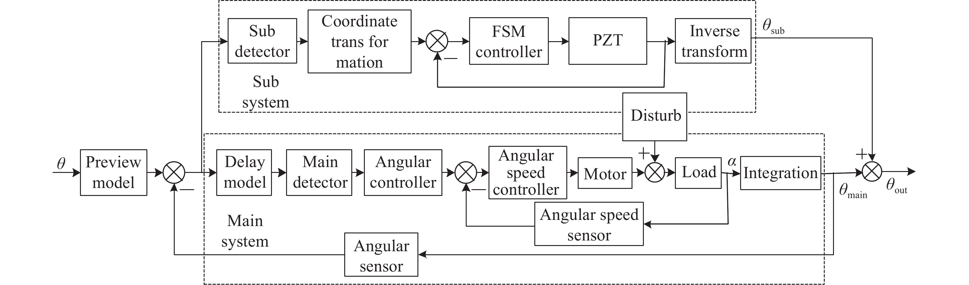
全回路跟踪系统由预瞄模型、主轴系统和从轴系统组成，系统原理图如图1所示。

图  1  复合轴伺服系统结构原理图

Figure 1.  Schematic diagram of compound axis servomechanism structure

控制结构图如图2所示。从图2可以看出，主轴系统由滞后环节、主轴探测器模型、电机模型、负载模型、角速度传感器模型、角度传感器模型及角度控制器和角速度控制器组成；从轴系统由从轴探测器模型、坐标变换、快反镜模型及角度控制器组成。这里，控制器均选用经典PID控制方法，角度传感器和角速度传感器的传递函数假设为1，即认为实际系统输出与测量系统输出一致。其他环节数学模型依据常规器件性能选择。

图  2  全回路跟踪系统控制结构图

Figure 2.  Whole-loop tracking system control structure diagram

电机选用直流力矩电机，系统采用PWM电压调速，因此可以得到系统的电平衡、力平衡方程，如公式(1)~(5)所示：

式中：u为调制电压；R₀为电机驱动总电阻；I表示流过电机绕组电流；L为电机绕组电感；${{\rm{d}}I / {{\rm{d}}t}}$为微分算子；E为电机绕组反电动式；J为电机及负载转动惯量；ω为电机负载角速度；f_m为机械阻尼；M为电机输出力矩；T_f(ω)为摩擦力矩；C_e为反电势常数；C_m为力矩常数；R为电机绕组电阻；R_q为驱动芯片内阻。在此基础上进行线性化处理，假设摩擦总阻系数f_m是不变的，进行拉式变换可得频域方程：

由系统框图求得系统闭环传递函数为：

因为电机电气时间常数${T_L} = {L / R}$，电机机械时间常数${T_M} = {{JR}/ {{C_e}{C_m}}}$且电机机械时间常数一般远远大于电气时间常数，可将公式(10)简化为：

预瞄模型为目标进入粗跟踪视场前的预先指向过程。机载激光武器跟踪系统实际工作中，由雷达等上游机构发送目标角度，该角度往往大于主轴探测器视场角，即此时目标处于主轴探测器视场外，需要控制机构旋转一定角度使目标进入主轴视场内后再进行复合轴控制。控制机构闭环传递函数${G_{VB}}\left( s \right)$为：

式中：${K_{si}}$${K_{sp}}$为PI控制参数。

预瞄模块的输出为${\theta _p}$，其表达式为：

式中：$\theta $为输入角度值。

图3(a)和(b)为预瞄模块功能对比图，目标初始位置为1.57 rad，预瞄过程时间为0.6 s。不采用预瞄模块的仿真系统在初期超调为38.71%，而采用预瞄模块的仿真系统没有超调，更符合实际工程情况。

图  3  预瞄模块功能对比图

Figure 3.  Preview model function comparison chart

由于脱靶量的输出中要经过光电扫描、A/D、D/A、图像识别算法等，使得输出的脱靶量滞后目标成像1~2帧，这里以2帧延迟为例，滞后时间约为20 ms。仿真平台中，直接使用延迟函数，作为滞后环节。

从轴系统是由压电陶瓷驱动的一块快速反射镜，通过光束在空间上的转动，来实现主控系统残余误差的补偿。仿真假定从轴系统探测器选用1 kHz的高帧频CCD，采用压电陶瓷驱动，传递函数的形式如标准二阶系统，根据实际工程经验可以将快反镜的数学模型${G_m}\left( s \right)$设为：

另外采用高速处理器后，图像跟踪器的纯滞后时间τ远小于采样周期T，所以可以忽略系统的纯滞后时间。

若假设驱动器与反射镜的接触点与镜面中心的距离为l，驱动器运动距离为d，镜面的旋转角度为${\theta _d}$，那么经过镜面的光线改变角度为2${\theta _d}$，所以反射比为2。坐标变换公式为：

由于进入子控系统的脱靶量非常小，一般在500 μrad以下，所以可将公式(15)近似为公式(16)：

探测器模型主要考虑最小分辨率因素，采用阶梯函数使得主系统探测器最小分辨率为50 μrad，子系统探测器最小分辨率5 μrad。数学公式为：

式中：ff为最小分辨率；θ为输入角度；θ_r为输出角度。

建立ADRC控制器。跟踪微分器方程表达式为：

式中：$h$为仿真时间间隔；${v_1}$为系统输入的跟踪信号；${v_2}$为输入的1阶微分信号；${f_s}$为系统的2阶微分信号；$u(t)$为输入信号；$r$为跟踪微分器的快速因子。

5阶扩张状态观测器表达式为：

式中：y为实际输出；${{\textit{z}}_1}$为对系统输出的估计；${{\textit{z}}_2}$为对系统输出1阶的估计；${{\textit{z}}_3}$为对系统扰动的估计；${\; \beta _{01}}、 {\; \beta _{02}}、 $$ {\; \beta _{03}}$为权重因子。

非线性控制器表达式为：

式中：${b_{01}},{b_{02}}$为非线性控制器的权重因子；${\alpha _1},{\alpha _2}$为非线性饱和因子；$theta$为切换阈值。$fal(e,\alpha ,theta)$的表达式为：

因为复合轴系统的主轴系统和从轴系统的输出是线性累加的，故两个系统的稳定性互不干涉，可分别验证主轴系统和从轴系统的稳定性。并且由于主轴系统中包含非线性函数，文中采用系统辨识后得到的近似线性系统，并通过计算系统零极点来判断系统稳定性。采用下文模型参数，利用最小二乘法可辨识出系统的参数模型，系统参数模型表达式为：

在将离散的参数模型，转换为连续模型，可以得到如公式(23)所示的连续参数模型：

据此，可以得到公式(23)所示系统和原始辨识系统的Bode对比图，如图4所示。

图  4  辨识系统与原系统对比Bode图

Figure 4.  Comparison of Bode diagram between identification system and original system

由Bode图可以看出，辨识精度较高，再通过仿真软件分析，辨识精度达到99.29%，几乎和原系统在2~200 Hz段内的频率特性一致。连续参数模型经过化简可得:

公式简化系统的闭环极点为：

由系统闭环极点可以得出系统稳定。

直升机初始地理坐标为北京的某坐标（北纬39.9°，东经116.3°），距离海面高度500 m缓慢飞行，北向初始速度为40 km/h，东向初始速度为30 km/h，且运动速度设定不变。侧向来袭导弹的速度为2 Ma（680 m/s），高度为3000 m。发现距离为20 km，一直向正北飞行，仿真时间为60 s。直升机和导弹的坐标关系如图5所示。

图  5  直升机和导弹的坐标关系图

Figure 5.  Coordinate diagram of helicopter and missile

依据第1节建立的数学模型和此场景假设，搭建图5中的MatLab/Simulink仿真平台。主轴系统角位置回路采用三阶自抗扰控制器，角速度回路控制器选用PID控制器，从轴系统的控制器采用经典PID控制，仿真参数设置如下：主轴系统频率f₁=100 Hz，从轴系统频率f₂=1000 Hz，主轴角度控制器自抗扰控制器参数选择如下：跟踪微分器步长h=1/100 s，跟踪微分器快速因子r=50，扩张状态观测器参数β₀₁=40，β₀₂=200，β₀₃=0.05，非线性控制器参数${\alpha _1=0.6}$，${\alpha _2=1.2}$，b₀₁=3，b₀₂=0.001，$theta$=0.8，主轴角速度控制器k_vp=40，k_vi=200，k_vd=0，因为电机电气时间常数${T_L}$=0.0015，电机机械时间常数${T_M}$=0.22，假设驱动器与反射镜的接触点与镜面中心的距离为l=0.03，从轴控制器k_cp=0.5，k_ci=160，k_cd=0，压电陶瓷放大系数k_p=15。

按照以上仿真参数搭建控制仿真系统，经测试，主轴系统角速度环开环截止频率为43.8 rad/s (6.97 Hz)，相位裕度为61°，幅值裕度为8.6 dB，角速度环闭环带宽为106 rad/s (16.88 Hz)，主控系统闭环带宽为11 rad/s (1.75 Hz)，从轴系统的闭环带宽为43.3 Hz，从—主轴带宽比约为25。

按照图5中搭建的全回路跟踪系统控制仿真图，然后分别对该仿真系统进行功能仿真试验验证和虚拟场景试验验证。

功能仿真仅以β方向为例。给定β输入曲线，以此验证仿真系统功能，系统扰动以实际采集的某型运输机在β方向扰动。

图6为功能仿真试验曲线，由图6(b)可以看出，主轴系统的偏差标准差为125.6 μrad。再以主轴系统β方向的偏差信号作为从轴系统的输入信号，可以得到图6(c)所示的跟踪曲线和图6(d)所示的跟踪偏差，从轴系统的偏差标准差为5.16 μrad。由复合轴控制理论可知，从轴系统的输出偏差即为总系统的输出偏差^[8]，即总系统的偏差为5.16 μrad。由从轴系统和主轴系统的跟踪精度对比可知，采用复合轴控制方式其跟踪精度相较于传统PID控制方式，跟踪精度由125.6 μrad提高到5.16 μrad，提高25倍。

图  6  全回路跟踪系统控制仿真图

Figure 6.  Whole-loop tracking system control simulation structure

虚拟场景按照第2节设定内容，为低速飞行直升机预警跟踪高速来袭导弹的实战场景，搭建的仿真结构见图5，加入扰动因素，俯仰方向幅值10 (°)/s，周期为4 s的角速度扰动，偏航方向幅值为45°，周期为3 s的角速度扰动。按照此虚拟场景可以确定仿真系统输入曲线如图7所示。

图  7  功能仿真试验曲线图

Figure 7.  Function simulation test curve

由于俯仰轴和偏航轴之间不存在耦合，故可以将俯仰轴和偏航轴分开进行仿真试验。按照第2节内容完成仿真参数设定。得到如图8~图10所示的仿真结果曲线。由图9(d)和图10(d)可以看出，复合轴伺服系统在10 (°)/s，周期为4 s的速度扰动下，从轴系统俯仰轴的跟踪精度能够达到±2 μrad，故系统俯仰轴跟踪精度亦为±2 μrad；在45 (°)/s，周期为3 s的速度扰动下，从轴系统偏航轴的跟踪精度能够达到±5 μrad，故系统偏航轴跟踪精度亦为±5 μrad。

图  8  虚拟场景仿真输入曲线图

Figure 8.  Virtual scene simulation input curve

图  9  虚拟场景俯仰轴仿真输出曲线图

Figure 9.  Virtual scene simulation output curve of pitch axis

图  10  虚拟场景偏航轴仿真输出曲线图

Figure 10.  Virtual scene simulation output curve of yaw axis

文中主要针对机载激光武器高精度跟踪系统，采用自抗扰控制器和复合轴伺服控制结构相融合的方式，通过建立预瞄模型、探测器模型、快速发射镜模型等数学模型，搭建完整的仿真系统。并通过功能验证试验和虚拟场景仿真试验验证文中搭建的仿真系统，其中功能验证试验扰动数据以某型运输飞机实际采集扰动数据为依据，仿真验证系统跟踪精度为5.16 μrad。虚拟场景仿真试验假定一种常见作战场景，在10(°)/s，周期为4 s的速度扰动下，系统俯仰轴跟踪精度为±2 μrad；在45(°)/s，周期为3 s的速度扰动下，系统偏航轴跟踪精度为±5 μrad，其跟踪精度相较于传统PID控制，跟踪精度提高25倍。

笔者课题实物平台已完成初步装调，目前正在进行光轴一致性调试工作，未来拟在实物平台上完成本课题控制算法的试验验证工作，主要是在六自由度摇摆台上，验证在典型扰动条件下，系统的稳定精度和跟踪精度指标。