


-
电厂、港口、钢厂、矿山作为主要的散货集散基地,在企业发展中有着重要的位置,目前国家正在大力提倡环境保护,对于钢厂、港口、电厂等污染较大的原料场进行封闭式管理,由于料场封闭,飘散的大量的粉尘,操作人员无法在现场进行设备操作,如何在恶劣的工作环境下高效、快速的完成散货的集散是这些企业进行经济规划、提高生产效率、合理安排生产计划的关键。对于如何有效地减少人工干预、提高生产效率、实现设备自动堆取作业是企业亟需解决的问题[1]。
随着钢厂、港口建设水平的提高、控制信息技术的迅猛发展,国内钢厂、港口对生产效率、自动化水平、节能减排、人员成本等提出了更高的要求,对钢厂、港口建设的全自动生产系统提出了新的需求。
在国外,煤炭(散货)装卸船全自动生产系统起步相对较早,从2002年荷兰鹿特丹EMO港建成投产,至2012年已建成投产的煤炭(散货)装船自动化港口已有8家。
在国内,近年来随着技术进步,特别是信息技术、控制技术突飞猛进的发展,自动化成本相对降低,制约煤炭装卸船自动化码头发展的瓶颈逐步得以克服,煤炭装船自动化码头整体呈现加速发展的势头。如天津港、曹妃甸、黄骅港等煤炭装船港口已经开始了自动化研究和应用。
近年来随着传感器、机器视觉、人工智能等技术的飞速发展,利用工业相机、激光雷达、三维扫描仪等视觉传感器设备进行数据采集,实现目标定位、识别、三维重建指导执行机构实现自动化作业完成闭环控制的应用越来越广泛。在国外基于LiDAR技术的堆取料自动控制已经有了很大的发展,而我国该项技术在堆取料机应用较晚与发达国家还存在一定的差距。特别是在封闭式料场中由于GPS系统在室内的定位精度较差,定位系统主要采用的是一些传统的传感器,精度误差大大高于室外采用GPS定位的方式,为了解决这些问题,文中是以首钢京唐封闭式料场无人化控制系统改造升级项目为依托,针对现代斗轮机的作业要求和特点,研发了一套基于LiDAR技术的散货料场堆取料机自动控制系统,通过对封闭式料场进行三维重建完成斗轮堆取料机的无人化控制和料场的可视化管理[2]。现场测试证明,该系统在保证作业安全同时的同时,具有误差低、稳定性强、实时性高等特点。
-
文中所提系统在堆取料机上配备了高性能的工业计算机,即机上服务器(CPC)做为核心计算单元,其主要作用是负责采集并处理位置传感器提供的定位数据、扫描仪提供的点云数据、与PLC进行数据交换,通过中控下发的作业计划以及扫描仪采集的点云数据进行实时建模,分析料堆的位置、形状等信息,找出合适的取料或者堆料位置,生成作业指令,通过PLC下发执行机构,指导堆取料机完成自动作业,同时将最新的三维数据传送的中控服务器(IDC)中,提供给中控可视化终端显示,系统架构如图1所示
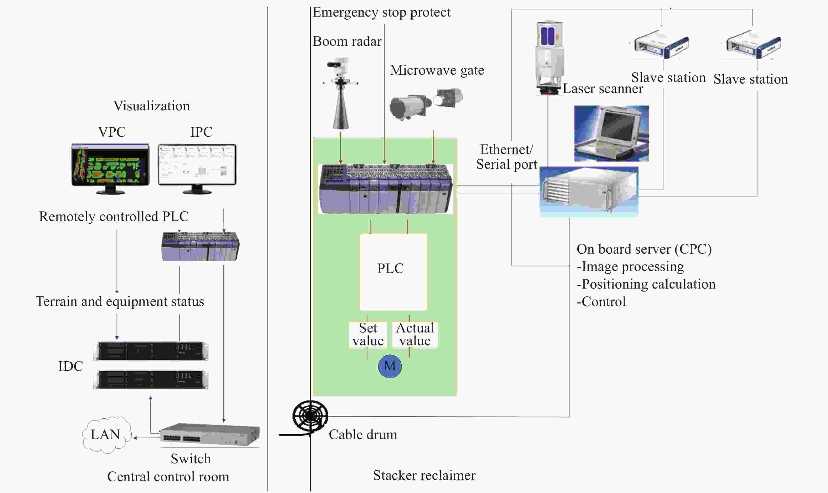
图 1 系统架构图
Figure 1. System architecture diagram
-
坐标系建立目的是为了求解各个坐标系之间的变换关系,能使数据还原到同一坐标系下,子坐标系包括:激光扫描仪坐标系Claser;俯仰机构坐标系Cpitch;回转机构坐标系Cyaw和轨道坐标系Crail(全局坐标系)。
轨道坐标系的选择与建立:设定设备沿轨道方向的走行为X轴、与轨道平面垂直的轴为Z轴、Y为X轴与Z轴的叉积,轨道原点定义为轨道端部的起点位置设定该位置的坐标在全局坐标系下的值为(0 m, 62 m, 0 m);全局坐标系与轨道坐标系方向一致,只是将全局坐标系原点位置平移沿Y方向平移62 m,全局坐标布置如图2所示。

图 2 全局坐标系布置图
Figure 2. Global coordinate system layout
定义Claser~Cpitch,Cpitch~Cyaw,Cyaw~Crail的变换为RT1,RT2,RT3,变换矩阵M由两部分组成,包括:R为旋转矩阵、T为平移矩阵,这两部分为主要的标定参数,设备在运动过程中的姿态数据利用走行位移传感器、回转和俯仰角度传感器反馈值给出,包括了走行距离、回转角度、俯仰角度,通过位置反馈值和扫描数据进行联合标定,堆取料机高29.86 m,臂架长36.6 m,尾车长68.5 m,斗轮直径为9 m,扫描仪安装在堆取料机顶部平台上,检测俯仰运动的倾角传感器与扫描仪安装在同一个平台,检测回转角度运动的传感器安装在回转机构,各坐标系建立如图3所示。

图 3 各坐标系的建立
Figure 3. Establishment of each coordinate system
标定流程原理:
(1)建立全料场全局坐标系,并在全料场确定3个及以上不共线目标点,文中目标点为4个标定球的球心,测量4个标定球的球心在全局坐标系下的坐标值;
(2)标定球为特殊定制,其半径为(24±1) cm,其的摆放位置在距离扫描仪直线距离70~120 m的任意位置,但要求在设备进行回转和俯仰运动时不被遮挡;
(3)扫描不同回转角度、俯仰角度下的标定球的轮廓点云数据,已知标定球的半径,各个球心之间的相对位置、球心到水平面的距离以及对每个球的曲率测量等为约束条件,进行提取球体表面的点云数据,提取结果如图4所示。
(4)根据球体表面数据采用最小二乘进行求解,公式(1)中的x、y、z为采集的球体表面坐标值,a、b、c,R为待求的球心坐标和半径。
$$\begin{array}{l} \\ \underbrace {\left[ {\begin{array}{*{20}{c}} {2{\rm{x}}}&{2y}&{2{{{\textit{z}}}}}&1 \end{array}} \right]}_A\underbrace {\left[ {\begin{array}{*{20}{c}} a \\ b \\ c \\ {d} \end{array}} \right]}_X = \underbrace {{x^2} + {y^2} + {{\textit{z}}^2}}_B \end{array} $$ (1) $${R^2} = {d} + ({a^2} + {b^2} + {c^2})$$ (2) $$X = {\left( {{A^{{\rm{ - }}1}}{\rm{·}}A} \right)^{ - 1}}{\rm{·}}A{\rm{·}}B$$ (3) 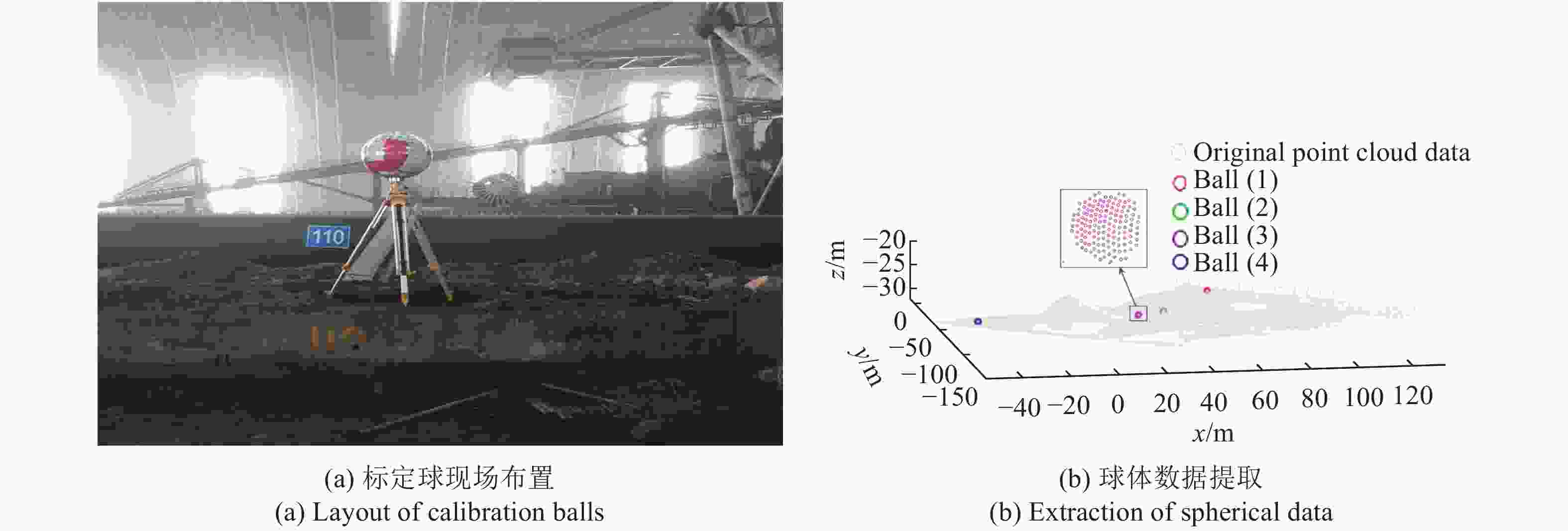
图 4 球体表面特征点提取
Figure 4. Feature point extraction of sphere surface
在全料场点云数据中对球体表面特征点的提取,根据提取的特征点求解出47组不同位姿下的球心坐标中,表1中写出了部分数据。
表 1 球心坐标计算
Table 1. The calculation of spherical center coordinates
Pose data rotation/(°), Pitch/(°), Travel/m Spherical coordinates/m [0.926, −4.124, 89.344] [−64.74, −10.273, 31.496]、[−37.625, 47.591, 28.838]、
[−26.578, 54.498, 28.758]、[37.375, 53.581, 29.715][11.309, −4.123, 89.344] [−63.213, −22.81, 32.29]、[−47.015, 38.96, 29.121]、
[−37.423, 47.749, 28.891]、[25.659, 58.433, 29.122][13.374, −4.125, 89.344] [−62.656, 25.153, 32.455]、[−48.621, 37.131, 29.181]、
[−39.326, 46.258, 28.923]、[23.338, 59.108, 29.015][29.1, −4.134, 89.344] [−55.534, −42.707, 33.695]、[−58.839, 21.039, 29.91]、
[−52.39, 32.263, 29.433]、[4.471, 61.561, 28.384]··· ··· ··· ··· [−10.307, 4.129, 89.344] [−63.791, 3.635, 30.671]、[−25.7, 54.933, 28.684]、
[−13.533, 59.511, 28.783]、[48.973, 45.927, 30.479][−22.542, −4.141, 89.344] [−59.717, 17.968, 29.908]、[−11.577, 60.013, 28.738]、
[1.289, 61.894, 29.009]、[59.388, 35.452, 31.381]采用Rodrigues形式将R表示为R(k, θ),k1为回转轴、k2为俯仰轴、k3为扫描仪与大机安装位置的固定关系,θ为不同位姿下回转或俯仰轴所对应的角度值,μi,j为第i个位姿下第j个球的在扫描仪坐标系下的坐标值,t为与k对应的平移量,Gcj为第j个球在料场坐标系下的坐标值,矩阵M为扫描仪坐标系转俯仰坐标系,俯仰坐标系转回转坐标系的一个综合表达式,全局标定归结为如公式(4)所示的优化问题,采用列文伯格-马夸尔特(LM)算法进行优化。
$$\begin{split} &M = \\ &\left[ {\begin{array}{*{20}{c}} {{R_{i,j}}\left( {{k_3},{\theta _3}} \right)}&{{t_3}} \\ 0&1 \end{array}} \right]\left[ {\begin{array}{*{20}{c}} {{R_{i,j}}\left( {{k_2},{\theta _2}} \right)}&{{t_2}} \\ 0&1 \end{array}} \right]\left[ {\begin{array}{*{20}{c}} {{R_{i,j}}\left( {{k_1},{\theta _1}} \right)}&{{t_1}} \\ 0&1 \end{array}} \right] \end{split}$$ (4) $$F\left( {{k_1},{k_2},{k_3},{t_1},{t_2},{t_3}} \right) = {\rm{argmin}}\left\{ {\sum\limits_{{i} = {\rm{1}}}^n {\sum\limits_{{j} = {\rm{1}}}^{\rm{4}} {{{\left\| {M{\mu _{i,j}} - G{c_j}} \right\|}^2}} } } \right\}$$ (5) 采集47组不同位姿的扫描仪数据进行分析;目标球的全局坐标如表2所示。
表 2 标定球全局坐标值
Table 2. Global coordinate value of calibrated sphere
Ball number Global coordinate value/m Ball (1) [123.295,660.216,0.847] Ball (2) [159.001,606.504,0.743] Ball (3) [158.997,593.499,0.697] Ball (4) [124.305,539.784,1.376] 根据采集的数据计算出不同位置下的球心在扫描仪坐标系下的值,采用LM算法进行参数优化,解算结果如表3所示,根据标定结果对球心进行误差反算,如图5所示,在100 m处其结果偏差为±6 cm,满足控制精度控制。
表 3 标定结果
Table 3. Calibration results
Parameter Result k1 [−0.0241322356578230, −0.00848742929874968, −1.00345840212693] k2 [−0.00698639711665264, 1.00404411551583, −0.00687821749052725] k3 [0.442325868464691, 0.884651736929383, 0.147441956154897] t1 [89.4487452221133, 600.106793609578, 14.5859227389128] t2 [−4.96064857485726, 125.966577019193, −32.5089193040485] t3 [14.4040035283724, −126.590439618449, −13.5939620742438] RT1 [0.904785904567622, −0.427438292148760, 0.00592253298597620, 89.4487452221133;
0.427477318501016, 0.904737285802332, −0.00946857001315529, 600.106793609578;
−0.00130849501319894, 0.0110913504977723, 1.00066010049210, 14.5859227389128; 0, 0, 0, 1]RT2 [0.974304531826196, −0.00172950424822600, −0.226149808195282, −4.96064857485726;
0.00136899717336400, 1.00020826129429, −0.00175107953908600, 125.966577019193;
0.226152277853766, 0.00139615467203800, 0.974304493284483, −32.5089193040485; 0, 0, 0, 1]RT3 [−0.514141631719535, 0.857133272554982, 0.0313198916339447, 14.4040035283724;
−0.857115239068129, −0.514799526319354, 0.0183006737186152, −126.590439618449;
0.0318095817319255, −0.0174356181581603, 0.999341858289486, −13.5939620742438; 0, 0, 0, 1]M [−0.687440474398016, 0.725546765708434, −0.0374128045419695, 99.5824377170413;
−0.726505435812832, −0.686720289505128, 0.0315812806063315, 597.013205725566;
−0.00277799062244338, 0.0488814199127985, 0.998999137047828, −30.4820647473178; 0, 0, 0, 1]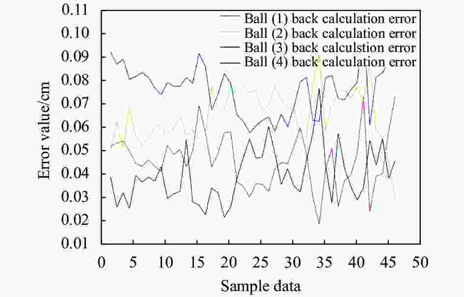
图 5 标准球反算误差
Figure 5. Back-calculation error of standard sphere
-
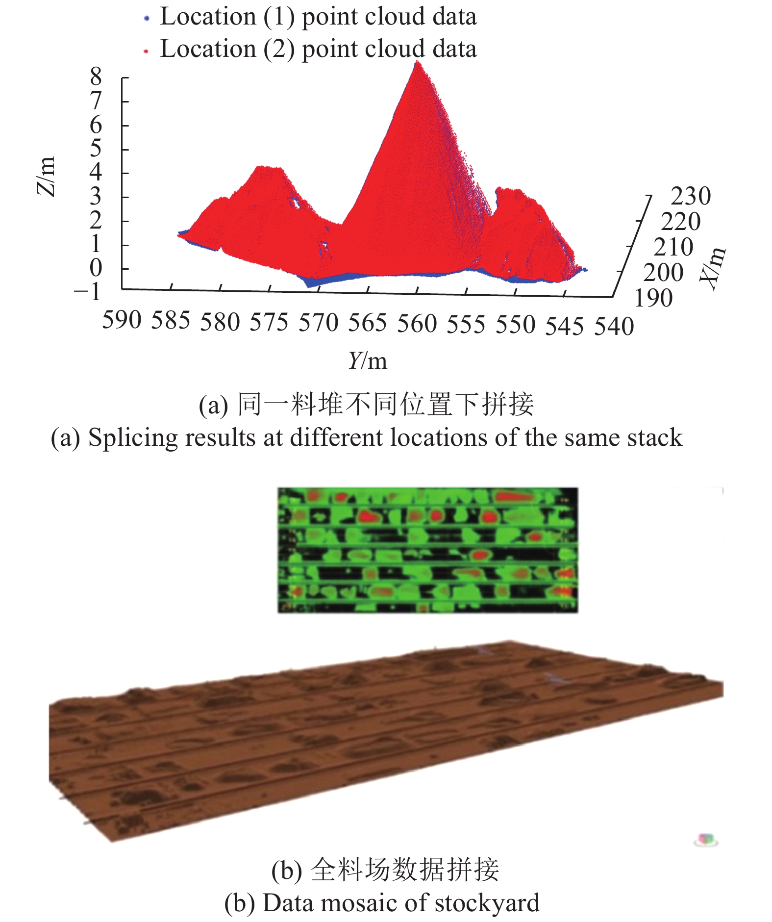
三维激光的发射是沿直线方向的,需要在不同角度对料堆进行扫描,将不同位置下的扫描数据还原到料场坐标系中,进行全料场点云数据的拼接,实现料场的可视化控制与管理。
想要求出两组点云的变换关系,必须要找到两站点云中三对或三对以上的特征点,由于标定球在标定完成后就会拆除,而且需要对点云进行实时拼接,不是等扫描完成后进行数据拼接,无法通过标定球作为同名点进行点云拼接,在三维点云拼接算法中,最经典的算法是Iterative Closest Point(ICP)算法[8-9],该算法是由Besl P和McKay提出,ICP算法原理是利用最小二乘来实现最优变换,该算法主要对数据进行后处理,难以进行数据实时处理,文中根据走行位移传感器、回转和俯仰角度传感器提供的实时姿态数据进行全料场点云数据拼接,每组姿态数据都带有时间标签,与扫描仪实时获取的点云的时间标签相对应,根据公式(4)完成点云数据拼接,拼接后的结果如图6所示。
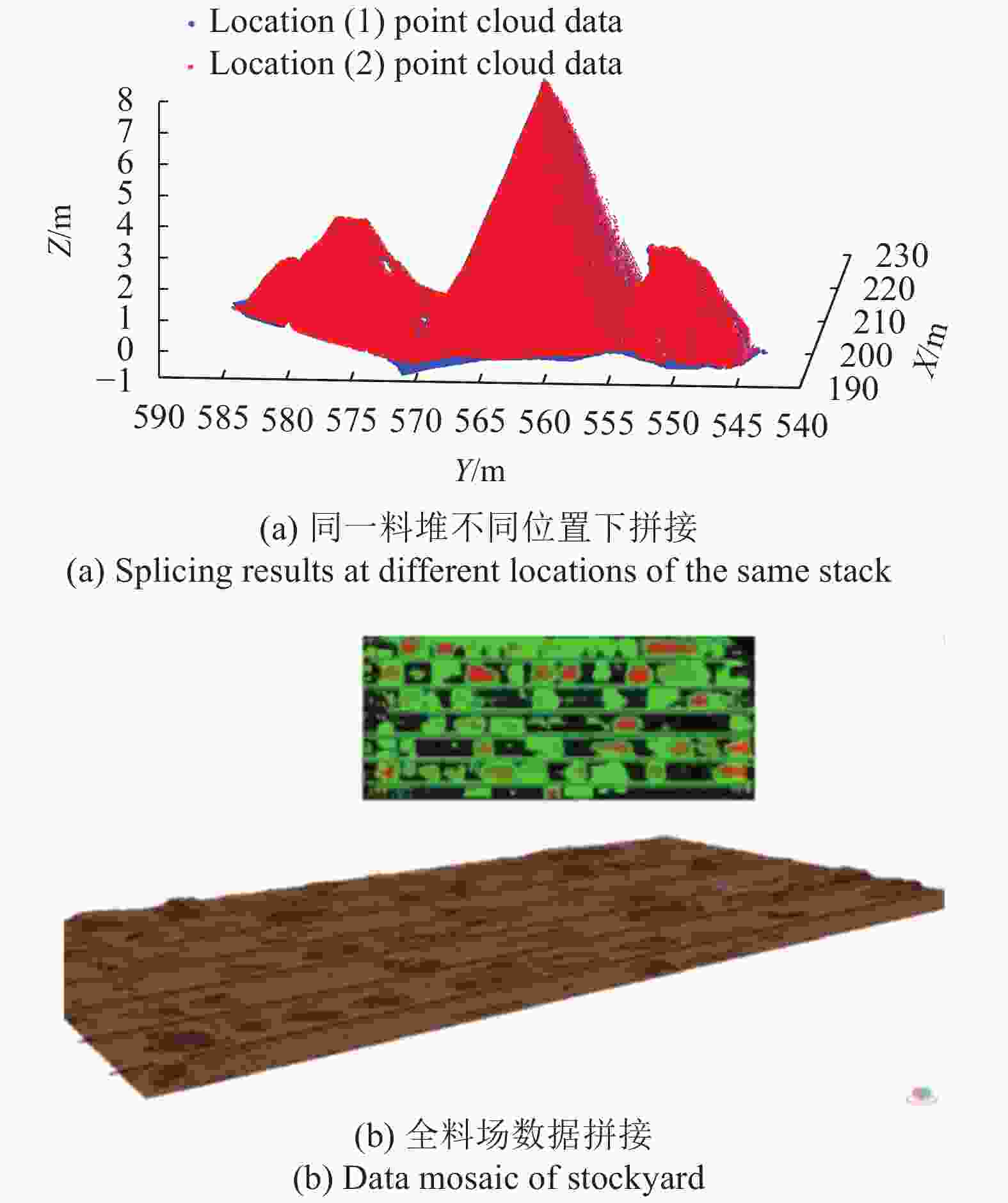
图 6 数据拼接效果图
Figure 6. Effect diagram of data mosaic
-
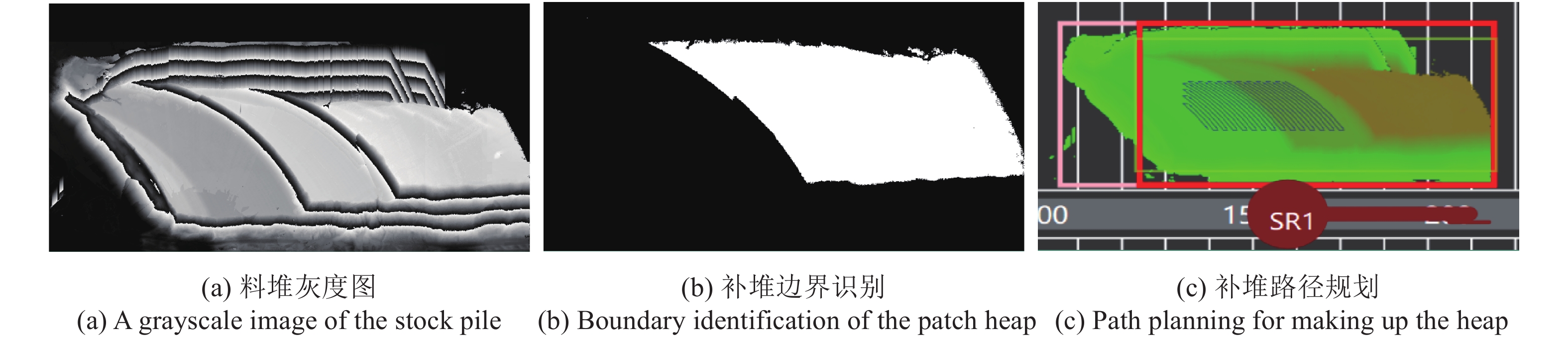
目前常见的斗轮堆取料机控制系统,大多利用可编程逻辑控制器(PLC)、PLC主从站、变频器、继电器、终端显示等,采用总线技术实现联合逻辑控制,并可以完成半自动和手动控制,由于PLC很难实现复杂的智能控制,难以解决无人值守操作,为此在文中所提系统中采用了基于LiDAR机器视觉技术,同时针对手动堆取料作业过程中作业随意性大、精度差、效率低等问题,依据堆取料机作业工艺特点[10],提出了一种基于视觉图像处理算法的作业路径规划算法,能够提前对设备的作业路径进行规划,并能视觉系统采集的料堆数据进行实时分析,实现路径的实时更新。路径规划算法流程:
(1)扫描目标作业区域获取点云数据;
(2)根据目标区域的范围、位置等限定条件,对料堆区域数据进行去燥,降低干扰数据对目标区域的影响;
(3)将料堆的点云数据转换为图像的像素点,X、Y为图像中的位置,Z为图像的灰度,转换后如图7(a)所示;

图 7 路径规划
Figure 7. Path planning
(4)为减小毛刺和漏洞对全局的规划造成的影响,采用5×5的卷积核对料堆的图像膨胀腐蚀处理;
(5)根据目标堆料高度对膨胀腐蚀处理后的图像进行二值化处理,再进行边缘提取,选取所有边界中的最大矩形边界,如图7(b)所示,计算出料堆上限边界的终止点;
(6)根据作业模式(堆料或取料)、作业方式(新堆、续堆、覆盖堆、分层分段取、分层整取)、识别出的料堆边界、安息角等参数计算出每次臂架的回转折返点的控制线;
(7)根据设备的臂长、回转步进角度、走行步进距离、折返点的控制线,计算出每条轨迹线具体的折返点的X、Y,如果在取料路径中发现有空洞会快速跳过该区域,在堆料路径中发现有料会造成碰撞会提前进行避让,设备的作业路径生成如图7(c)所示。
-
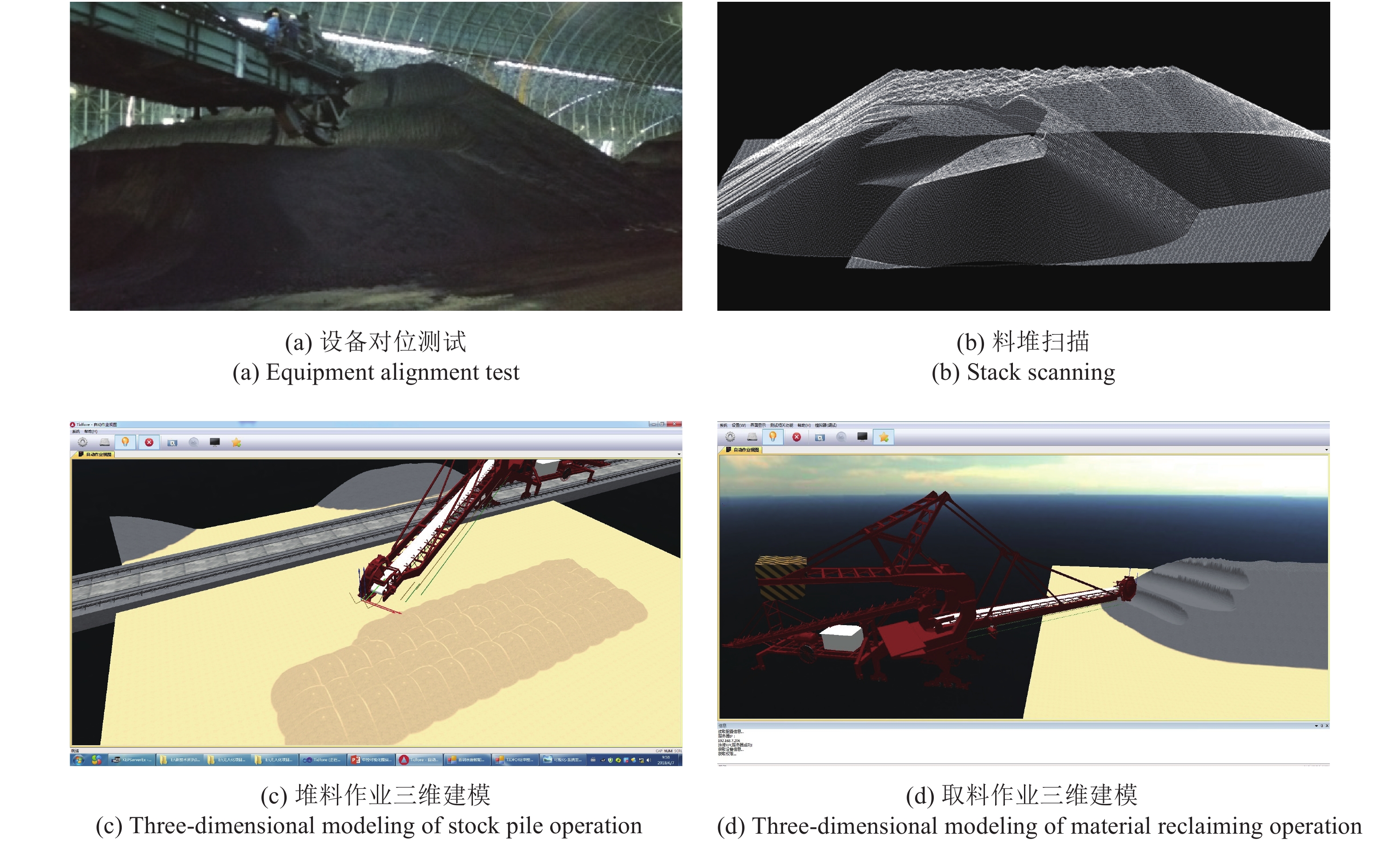
该系统以首钢京唐原料场无人化控制系统改造升级项目为背景,对系统进行综合测试,在接收到中控下发的作业任务后,进行一系列的处理,包括作业任务分析、目标作业区域扫描、料堆的三维重建、作业路径的生成、自动化堆取作业等无人化操作,现场测试过程如图8所示。
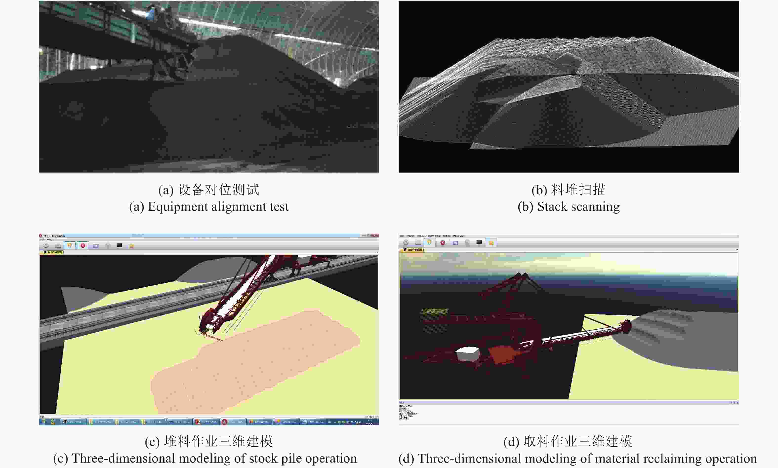
图 8 现场测试
Figure 8. Field test
-
通过研究LiDAR机器视觉在散料堆取料机全自动控制应用过程中的关键技术,有效解决了三维激光扫描仪在项目应用过程中的难点。基于设备自生位移传感器和角度传感器建立的全局标定模型,利用走行位移传感器、回转和俯仰角度传感器与标定球构成的标定点相结合的方式实现全局标定,完成了扫描仪坐标系到全局坐标系的转化,现场测试表明,在不同的大机位姿下对同一目标数据进行描仪,数据误差可控制在±10 cm以内,满足自动作业要求。在此基础上,设计开发出全料场2D和3D可视化终端、自动作业路径规划库集成于料场无人化系统,该技术在首钢京唐原料场堆取料机无人化操作自动控制系统项目中的到了应用和验证,项目性能指标达到国际同类型先进产品水平。
Research on key technologies of intelligent control system of bucket wheel machine in enclosed stockyard
-
摘要: 针对目前封闭式料场堆取料机工作环境恶劣、作业效率低、误差大、成本高等问题,设计了一套堆取料机智能控制系统,该系统基于LiDAR技术,通过扫描仪采集料堆表面点云数据,利用定位系统与扫描仪的联合标定,完成定位传感器反馈的姿态数据与扫描数据实时匹配,实现点云数据的处理和料三维重建,同时通过图像处理技术,提前预测作业路径来指导封闭料场中堆取料机完成自动作业。实验表明该控制系统控制提高了工作的效率,降低了作业成本。Abstract: Aiming at the problems of poor working environment, low operating efficiency, large operating error and high cost of the stacker and retractor in the enclosed stockyard, a set of intelligent control system for stacker and retractor was designed. The system was based on LiDAR technology, through the scanner to obtain stock pile surface point cloud data, the positioning system with the combination of scanner calibration was used to completethe real-time matching between the positioning sensor feedback profile data and scan data, realize the point cloud dataprocessing and 3D reconstruction of stock. Through image processing technology, the operation path was forecasted advance to guide the stacker and retractor to complete automatic operation in a enclosed stockyard. Experiment shows that the control system improves the work efficiency and reduces the operation cost.
-
Key words:
- calibration /
- LiDAR /
- path planning /
- image processing /
- machine vision /
- intelligent control
-
表 1 球心坐标计算
Table 1. The calculation of spherical center coordinates
Pose data rotation/(°), Pitch/(°), Travel/m Spherical coordinates/m [0.926, −4.124, 89.344] [−64.74, −10.273, 31.496]、[−37.625, 47.591, 28.838]、
[−26.578, 54.498, 28.758]、[37.375, 53.581, 29.715][11.309, −4.123, 89.344] [−63.213, −22.81, 32.29]、[−47.015, 38.96, 29.121]、
[−37.423, 47.749, 28.891]、[25.659, 58.433, 29.122][13.374, −4.125, 89.344] [−62.656, 25.153, 32.455]、[−48.621, 37.131, 29.181]、
[−39.326, 46.258, 28.923]、[23.338, 59.108, 29.015][29.1, −4.134, 89.344] [−55.534, −42.707, 33.695]、[−58.839, 21.039, 29.91]、
[−52.39, 32.263, 29.433]、[4.471, 61.561, 28.384]··· ··· ··· ··· [−10.307, 4.129, 89.344] [−63.791, 3.635, 30.671]、[−25.7, 54.933, 28.684]、
[−13.533, 59.511, 28.783]、[48.973, 45.927, 30.479][−22.542, −4.141, 89.344] [−59.717, 17.968, 29.908]、[−11.577, 60.013, 28.738]、
[1.289, 61.894, 29.009]、[59.388, 35.452, 31.381] 下载: 导出CSV
表 2 标定球全局坐标值
Table 2. Global coordinate value of calibrated sphere
Ball number Global coordinate value/m Ball (1) [123.295,660.216,0.847] Ball (2) [159.001,606.504,0.743] Ball (3) [158.997,593.499,0.697] Ball (4) [124.305,539.784,1.376]
下载: 导出CSV
表 3 标定结果
Table 3. Calibration results
Parameter Result k1 [−0.0241322356578230, −0.00848742929874968, −1.00345840212693] k2 [−0.00698639711665264, 1.00404411551583, −0.00687821749052725] k3 [0.442325868464691, 0.884651736929383, 0.147441956154897] t1 [89.4487452221133, 600.106793609578, 14.5859227389128] t2 [−4.96064857485726, 125.966577019193, −32.5089193040485] t3 [14.4040035283724, −126.590439618449, −13.5939620742438] RT1 [0.904785904567622, −0.427438292148760, 0.00592253298597620, 89.4487452221133;
0.427477318501016, 0.904737285802332, −0.00946857001315529, 600.106793609578;
−0.00130849501319894, 0.0110913504977723, 1.00066010049210, 14.5859227389128; 0, 0, 0, 1]RT2 [0.974304531826196, −0.00172950424822600, −0.226149808195282, −4.96064857485726;
0.00136899717336400, 1.00020826129429, −0.00175107953908600, 125.966577019193;
0.226152277853766, 0.00139615467203800, 0.974304493284483, −32.5089193040485; 0, 0, 0, 1]RT3 [−0.514141631719535, 0.857133272554982, 0.0313198916339447, 14.4040035283724;
−0.857115239068129, −0.514799526319354, 0.0183006737186152, −126.590439618449;
0.0318095817319255, −0.0174356181581603, 0.999341858289486, −13.5939620742438; 0, 0, 0, 1]M [−0.687440474398016, 0.725546765708434, −0.0374128045419695, 99.5824377170413;
−0.726505435812832, −0.686720289505128, 0.0315812806063315, 597.013205725566;
−0.00277799062244338, 0.0488814199127985, 0.998999137047828, −30.4820647473178; 0, 0, 0, 1]
下载: 导出CSV
-
[1] Zhang Ruilian, Wu Zhijian. Analysis on current status and intellectualization development tendency of stacker-reclaimer at home and abroad [J]. Mining & Processing Equipment, 2013, 41(6): 5-8. (in Chinese) [2] Jian Xin, Zhou Quan, Huang Huan. Application of 3D laser scanner to 3D modeling of bulk material yard [J]. Port Operation, 2018(1): 32-35. (in Chinese) doi: 10.3963/j.issn.1000-8969.2018.01.011 [3] Zhang Bai, Shi Zhaoyao. Three-dimensional scanning probe calibration method [J]. Journal of Beijing University of Technology, 2013, 39(4): 481-486. (in Chinese) [4] Wan Peng, Guo Junjie, Li Haitao, et al. Study on multiregion variable parameters method for 3D orthogonal scanning probe calibration [J]. Journal of Xi'an Jiaotong University, 2012, 46(7): 57-62, 114. (in Chinese) [5] Hu Yong, Wang Congjun, Han Ming, et al. 3D laser scanning measure system based on computer vision [J]. Journal of Huazhong University of Science and Technology(Nature Science), 2004, 32(1): 16-18. (in Chinese) doi: 10.3321/j.issn:1671-4512.2004.01.006 [6] Zheng Xuehan, Wei Zhenzhong, Zhang Guangjun. Expeditions calibration algorithm of visual tracking and measurement system with field coordinate system for moving target [J]. Infrared and Laser Engineering, 2015, 44(7): 2175-2181. (in Chinese) doi: 10.3969/j.issn.1007-2276.2015.07.036 [7] Li Zhe, Ding Zhenliang, Yuan Feng. Global calibration method for multi-vision measurement system with coplanar targets [J]. Optics and Precision Engineering, 2008, 16(3): 467-472. (in Chinese) doi: 10.3321/j.issn:1004-924X.2008.03.016 [8] Besl P, McKay N. A method for registration of 3-D shapes [J]. IEEE Transactions on Pattern Analysis and Machine Intelligence, 1992, 14(2): 239-256. doi: 10.1109/34.121791 [9] Dai Jinglan, Chen Zhiyang, Ye Xiuzi. The application of ICP algorithm in point cloud alignment [J]. Journal of Image and Graphics, 2007, 12(3): 517-521. (in Chinese) doi: 10.3969/j.issn.1006-8961.2007.03.023 [10] 吴颖昕. 斗轮堆取料机堆取料工艺与控制方法的研究[D]. 辽宁: 东北大学, 2009. Wu Yingxi. Research on the technology and control method of Bucket Wheel Stacker Reclaimer[D]. Shenyang: Northeast University, 2009. (in Chinese) -

 点击查看大图

图(8) / 表(3)
计量
- 文章访问数: 238
- HTML全文浏览量: 111
- PDF下载量: 25
- 被引次数: 0


