


-
大型结构的垮塌或失效会导致巨大的人员和经济损失。由于结构老化和不可预测的外因影响,具有全寿命周期监测能力的结构健康监测(Structural Health Monitoring, SHM)系统成为优化结构运行和养护策略,避免灾难性事故发生的有效方式。因此,近年来SHM被广泛应用于桥梁、隧道、大坝等大型结构缺陷识别、养护设计和验证工程中[1-3]。
随着数据挖掘和计算技术的进步,SHM系统已超越既定功能,而被赋予结构损伤检测、可靠性评价和剩余使用寿命估计[4-6]等新使命。由于在役SHM系统长期、连续工作于野外环境,对SHM系统的性能评价面临诸多难题,例如离线评价方式可能导致的监测中断、在线评价的不可控环境影响等。
基于光纤光栅技术的应变监测系统因其高灵敏度和布设的灵活性等优点,成为当前结构监测应用的热点[7-9]。系统采用光纤应变传感器,以刻有光栅的光纤作为感知应变的弹性元件,结构变形传递至光纤,通过检测光纤物理参数的变化来实现结构的应变测量。这种原理决定了结构应变监测的准确性和连续性对传感器的安装状态具有较强的依赖性。因此,在役系统的性能评价不能脱离现场条件。
在SHM系统的运行状态分析方面,Li Lili等提出了一种利用广义似然比和相关系数进行传感器故障检测的方法,在长江大桥上进行了人工故障传感器检测和分类验证测试,可实现多种传感器故障的在线诊断[10]。彭璐等利用参考传感系统的动态测量结果,提出了一种基于分层正交人工蜂群(HOABC-NN)神经网络的方法,实现了电阻应变传感系统的原位标定[11]。然而,现有工作仍难以解决在役应变监测系统测量性能的量化评价问题,对支撑SHM系统在野外复杂工况下的长期性能研究尚存不足。
文中以广泛应用的光纤式应变监测系统为例,提出了基于数据序列特征分析的在役监测系统性能评价方法。该方法以参考系统建立数据比较基准,通过自然激励条件下的匹配数据序列的结构特征分析,建立性能评价模型。通过仿真数据和实际SHM系统验证了该方法的可行性。
-
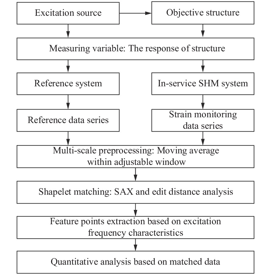
两套正常性能的传感系统对同一物理量进行测量时,所获得的数值序列应当具有良好的相似度。由于结构监测现场环境的复杂性,以及大型结构受激响应的不可控性,这一原理应用于在役SHM系统的评价时,需要建立完善的技术框架、数据处理及评价策略。图1所示为文中所提方法的技术框架。该技术框架基于参考测量系统和在役监测系统对同一(或相近)物理量进行同步测量的基本条件。因此,参考测量系统与在役监测系统的传感器应同向近距离并列安装。

图 1 技术框架
Figure 1. Technical framework
图1中,目标结构物在自然激励条件下,产生应变响应,在役应变监测系统和经过计量溯源的参考测量系统分别获取该结构响应的测量结果。为去除干扰因素的影响,通过加窗的均值滤波进行序列数据处理,形成具有不同细节层次的数据序列。然后,经过典型形态子段的查找匹配,得到两原始数据序列的初始匹配关系,解决因同步时间误差导致的序列错位问题。进一步,以初始匹配位置为起点,双向搜索提取峰值和谷值特征点,以特征点为约束条件,匹配形成用于量化分析的同名点序列。最后,建立分析模型,计算可量化的性能指标。
对于SHM系统性能的评价,采用分步评价的策略,流程图如图2所示。在预处理、形态子段匹配和特征点提取过程中,均可实现参数调节,以得到不同尺度或细节层次的评价结果。

图 2 系统性能评价策略
Figure 2. System performance evaluation strategy
在形态子段匹配过程中,若在一定时间区间和步长条件下得不到良好的匹配,即表明两序列的一致性较差,可以初步判断光纤应变监测系统的性能不佳。在得到良好的形态子段匹配结果的情况下,进一步通过特征点提取和同名特征点序列分析的方法计算系统性能的量化指标。
该评价方法中的可调节参数包括:均值滤波的窗口宽度、形态子段的长度和范围、符号化映射的步长等。
-
图1中,参考测值序列和应变监测值序列,本质上均为时间序列。参考文献[12]方法在两个匹配序列的采样频率接近,且累积时程差异不大的情况下,取得了较好的效果。但对于两个较长的时间序列,在序列起始位置相差较远、序列的尺度差异较大的情况下,需进行匹配算法优化。
文中算法基于符号聚集近似(Symbolic Aggregate approXimation, SAX)的表示方法[13],通过分段均值到字符的映射,用离散的低维数据表示典型时间序列的形态特征。Ye Lexiang在参考文献[14]中利用SAX方法对时间序列形态子段(Shapelets)进行表征,实现了快速分类,解决了传统分类算法(如最近邻算法及相关优化算法)难以应用到时间序列集上的问题。
文中利用字符化表征思想,在参考量值序列中,选取包含典型特征的子序列作为Shapelet,并利用SAX将实数集中的形态匹配问题转化为基于字符集的形态匹配问题。分别记参考量值序列和应变监测值序列为P和Q,则上述匹配算法的实现过程如下:
Step 1:采用加窗均值滤波对P和Q原始数值序列进行预处理;
Step 2:在P序列中选取具有典型特征的序列形态子段作为一个Shapelet,记为S;
Step 3:根据参考测量系统和在役监测系统的测量频率设定步长
${l_1}$ 和${l_2}$ ,利用SAX方法对S和Q进行字符化表示;Step 4:利用基于编辑距离的相似性特征查找S在Q序列上的最佳匹配子段,并标记;
Step 5:以P序列的最佳匹配位置为起点,双向查找P和Q序列的峰值和谷值点,作为P和Q序列的匹配特征点;
Step 6:以匹配特征点为控制点,对相邻控制点间的数据进行精细匹配。
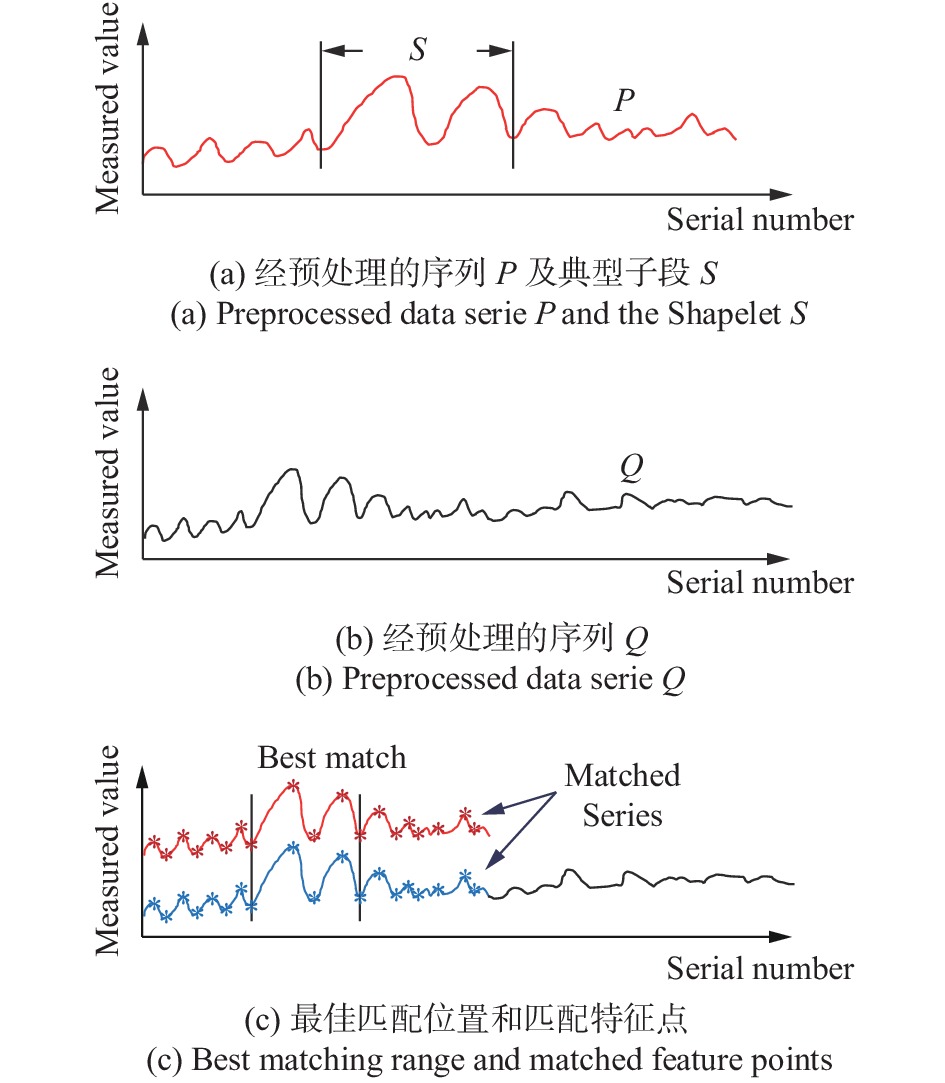
图3所示为匹配方法的实现过程。

图 3 所提序列匹配方法示意图
Figure 3. Schematic diagram of proposed series matching method
-
在参考量值序列
$P = {p_1},{p_2}, \cdots ,{p_{{n_1}}}$ 上选取一段长度为$k$ ,起始序号为$m$ ($0 \leqslant m < {n_1}$ )的子段作为Shapelet,记为:$S = {p_{m + 1}},{p_{m + 2}}, \cdots ,{p_{m + k}}$ 。设应变监测值数据序列为:$Q = {q_1},{q_2}, \cdots ,{q_{{n_2}}}$ 。对序列$S$ 和$Q\,$ 进行字符化映射,设步长分别为${l_1}$ 和${l_2}$ ,降维后的新序列分别表示为$S'$ 和$Q'$ :$$S' = {p'_1},{p'_2}, \cdots ,{p'_{[k/{l_1}]}},\;\;Q' = {q'_1},{q'_2}, \cdots ,{q'_{[{n_2}/{l_2}]}}$$ (1) 其中,
$S'$ 和$Q'$ 中第$i$ 项${p'_i}$ 和${q'_i}$ 由下式得到:$${p'_i} = \frac{{\displaystyle\sum\limits_{j = 1}^{{l_1}} {{p_{(i - 1) \times {l_1} + j}}} }}{{{l_1}}},\;\;{q'_i} = \frac{{\displaystyle\sum\limits_{j = 1}^{{l_2}} {{q_{(i - 1) \times {l_2} + j}}} }}{{{l_2}}}$$ (2) 且
${l_1}$ 和${l_2}$ 满足:$$\frac{{{l_1}}}{{{l_2}}} = \frac{{{f_1}}}{{{f_2}}}$$ (3) 式中:
${f_1}$ 、${f_2}$ 分别为参考系统和在役应变监测系统的测量频率。将所得新序列
$P'$ 和$Q'$ 中的数据分别映射到字符串,设序列$P'$ 和$Q'$ 中元素的数值区间分别为$[{V_{pL}}, $ $ {V_{pH}}]$ 和$[{V_{qL}},{V_{qH}}]$ ,若满足:$${p'_i} \in \left( {{V_{pL}} + \frac{{{V_{pH}} - {V_{pL}}}}{t} \times r,{\kern 1pt} {\kern 1pt} {V_{pL}} + \frac{{{V_{pH}} - {V_{pL}}}}{t} \times \left( {r + 1} \right)} \right)$$ (4) 则:
$${p'_i} \to CharSet[r]$$ (5) 即
${p'_i}$ 映射到字符集$CharSet$ 的第$r$ 个字符上。上式中$t$ 为字符集的字符总数,$r \in \left\{ {1,2, \cdots ,t} \right\}$ 。同理,当满足:$${q'_i} \in \left( {{V_{qL}} + \frac{{{V_{qH}} - {V_{qL}}}}{t} \times r,{\kern 1pt} \,{V_{qL}} + \frac{{{V_{qH}} - {V_{qL}}}}{t} \times \left( {r + 1} \right)} \right)$$ (6) 时,则:
$${q'_i} \to CharSet[r]$$ (7) 图4所示为字符映射过程,图中字符总数
$t = 5$ 。图中所示时间序列的映射值为“aabcbcdedbbba”。
图 4 字符映射示意图
Figure 4. Schematic diagram of character mapping
-
为了从应变监测值字符化序列中查找Shapelet的最佳匹配,利用编辑距离(Minimum Edit Distance,MED)作为度量两个序列相似程度的指标。编辑距离指两个字符串之间,由长度为
$m$ 的字符串${S_1}$ 转化为另一个长度为$n$ 的字符串${S_2}$ 所需要的最少单字符编辑操作次数。其中单字符编辑操作包含插入、删除和替换三种。以$edit(i,j)$ 表示${S_1}$ 的长度为$i$ 的子串到${S_2}$ 的长度为$j$ 的子串的编辑距离,则MED可通过以下递归运算得到。$$edit(i,j) = \left\{ {\begin{array}{*{20}{l}} {0, \;\;\;\;\;\;\;\;\;\;\;\;\;\;\;\; \;\;\;\;\;\;\;i = 0,j = 0} \\ {j, \;\;\;\;\;\;\;\;\;\;\;\;\;\;\;\;\;\;\;\;\;\;\; i = 0,j > 0} \\ {i, \;\;\;\;\;\;\;\;\;\;\;\;\;\;\;\;\;\;\;\;\;\;\;\; i > 0,j = 0} \\ {\min \left\{ \begin{array}{l} edit\left( {i - 1,j} \right) + 1, \\ edit\left( {i,j - 1} \right) + 1, \\ edit\left( {i - 1,j - 1} \right) + f\left( {i,j} \right) \\ \end{array} \right\},i > 0,j > 0} \end{array}} \right.$$ (8) 式中:当第一个字符串的第
$i$ 个字符不等于第二个字符串的第$j$ 个字符时,$f(i,j) = 1$ ,否则,$f(i,j) = 0$ 。定义两字符串之间的相似度SIM为:
$${\rm{SIM}} = 1 - {\rm{MED}}/\max (m,n)$$ (9) 式中:
$\max (m,n)$ 为两字符串的最大长度。易知,S和P的字符化序列的最佳匹配位置处,SIM将取得最大值。因此,这一匹配过程即转换为SIM最大值的求解过程。
-
经过匹配的应变监测值和参考测量值构成两个维度相等的向量,分别记为
$L = {L_1},{L_2}, \cdots ,{L_N}$ 和$Y = {y_1}, $ $ {y_2}, \cdots ,{y_N}$ (N为自然数)。由于参考测量系统是经过计量溯源的,其测值向量具有良好的准确性和可靠性。文中技术框架中,在役光纤应变监测系统与参考系统所测的为同一物理量在临近位置的分量。因此,光纤应变监测系统的计量性能与两向量的相似度具有正相关性。实验室条件下的线位移传感系统评测,通常采用多次循环、正反行程试验所得的测量值和参考值,以拟合残差的最大值计算基本误差,用于量化评价。然而,受在役应变监测系统的现场运行条件所限,实际试验过程是在不可控的被动激励条件下完成的,影响因素具有较大的随机性。从文中前期试验研究结果看,以拟合残差的最大值来表征在役应变监测系统的性能,不易得到稳定的量化评价结果,对监测系统的长期性能演变规律的研究是不利的。
文中提出,采用经过匹配的两组测值序列线性拟合残差(相对值)的包含概率为p的区间半宽度,来量化评价在役应变监测系统的性能。
对应变测量值和参考值序列
$L$ 和$Y$ 进行线性拟合,利用最小二乘法计算得到拟合直线方程${Y_i} = $ $ {Y_0} + K{L_i}$ 。斜率$K$ 及截距${Y_0}$ 的计算公式如下:$$K = \frac{{\displaystyle\sum\limits_{i = 1}^N {{L_i}{y_i}} - \overline L\sum\limits_{i = 1}^N {{y_i}} }}{{\displaystyle\sum\limits_{i = 1}^N {{L_i}^2} - \overline L\displaystyle\sum\limits_{i = 1}^N {{L_i}} }}$$ (10) $${Y_0} = \frac{{\overline y\displaystyle\sum\limits_{i = 1}^N {{L_i}^2} - \overline L\displaystyle\sum\limits_{i = 1}^N {{L_i}{y_i}} }}{{\displaystyle\sum\limits_{i = 1}^N {{L_i}^2} - \overline L\displaystyle\sum\limits_{i = 1}^N {{L_i}} }}$$ (11) 式中:
${Y_i}$ 为${y_i}$ 的拟合输出值;${Y_0}$ 为参比直线的截距;$K$ 为参比直线的斜率;${y_i}$ 为应变监测值序列的第$i$ 个匹配点的值;$\overline y$ 为应变监测值序列各匹配点的平均值;${L_i}$ 为参考测值序列的第$i$ 个匹配点的值;$\overline L$ 为参考测值序列各匹配点的平均值。根据参比直线方程求拟合输出值
${Y_i}$ 后,采用公式(12)作为计算基本误差的备选值。$${\delta _i} = \frac{{{y_i} - {Y_i}}}{{{Y_{{\rm{FS}}}}}} \times 100{\text{。}} ,\;\;i = 1,2, \cdots N$$ (12) 式中:
${Y_{{\rm{FS}}}}$ 为拟合直线上最大输入值${L_{\max }}$ 和最小输入值${L_{\min }}$ 所对应的输出值之差,即${Y_{{\rm{FS}}}} = K \cdot ({L_{\max }} - {L_{\min }})$ 。在役光纤应变监测系统的性能指标可表示为:
$${C_p} = HalfWid\{ {\delta _i}|p\,;\,\,i = 1,2, \cdots ,N\} \;\;$$ (13) 式中:p为包含概率,建议在90%~99%间取值。
-
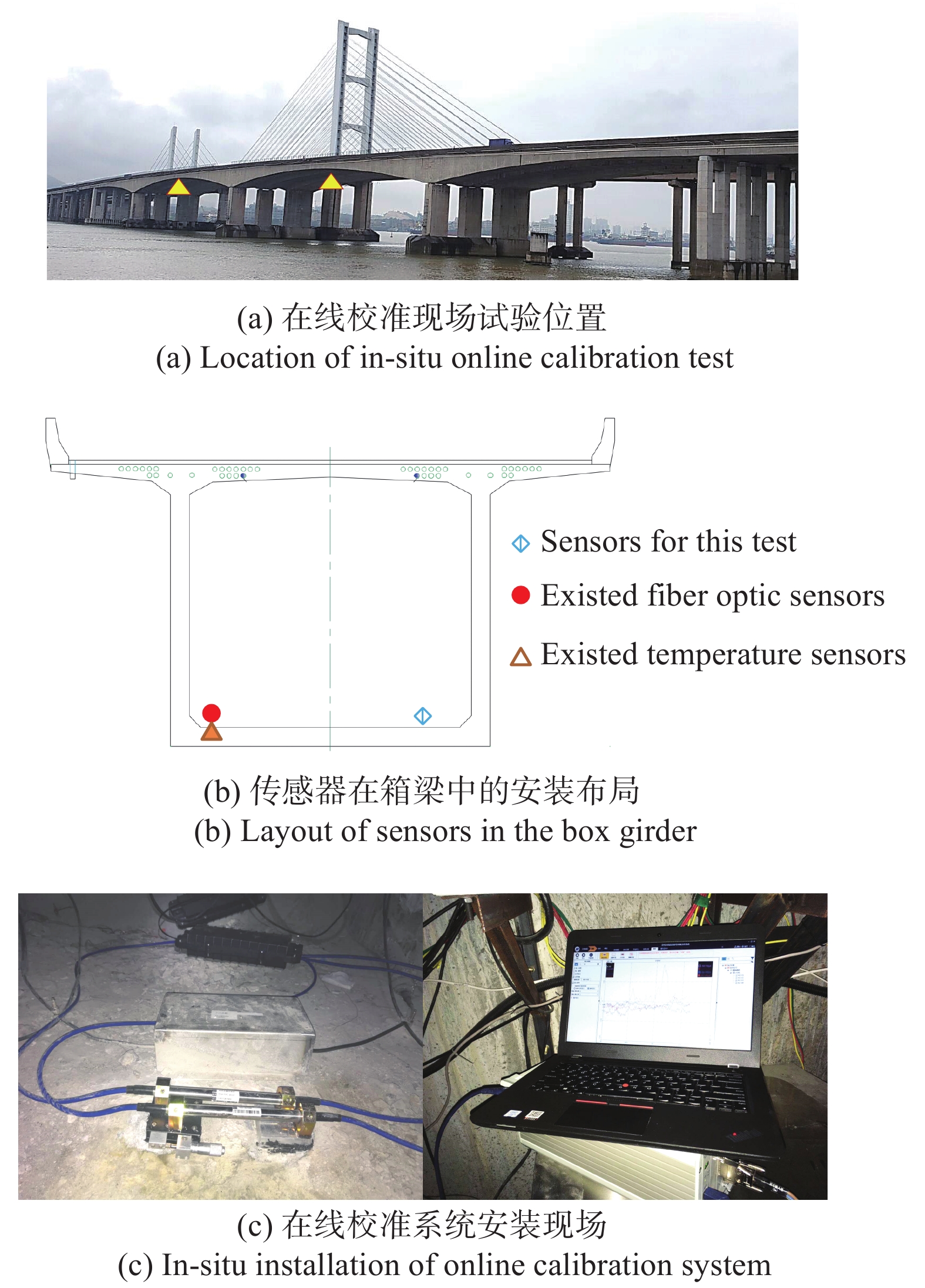
依托沈海高速(G15)佛山至开平段九江大桥(原桥),开展了文中方法的现场实证试验。在图5(a)中“△”标记位置的箱梁内侧布设光纤应变监测系统,传感器在桥梁箱梁截面内的布局如图5(b)所示,其安装状态如图5(c)所示。

图 5 现场验证及试验条件
Figure 5. In-situ verification and test conditions
现场试验所用光纤应变传感器的技术参数如表1所示。
表 1 光纤应变传感器参数
Table 1. Parameters of the fiber strain sensors
SN Stain coeff./
µε·nm−1Temperature coeff./
µε·nm−1Init. wavelength/
nm#669 778.0437 −789.5004 1553.151 #592 726.0287 −669.8661 1545.491 光纤应变数据采集采用SEN-01型光纤解调仪,测量波长范围1525~1565 nm,最大允许误差±0.5 pm,分辨力0.1 pm,采集频率1~100 Hz。
表1中,#669和#592传感器分别用于模拟在役应变监测系统和参考系统。测量频率分别设为15 Hz和20 Hz,通过调节两传感器的初始张紧状态,使其处于不同的测值区间。
-
在正常行驶车辆和自然环境的组合激励条件下,在役应变监测系统(SMS)与参考传感系统(RS)分别获取光纤应变监测序列数据,如图6所示。对原始数据按各自测量频率(Hz)数值的5倍设定滤波窗口宽度,得移动平均值序列,如图中虚线所示。
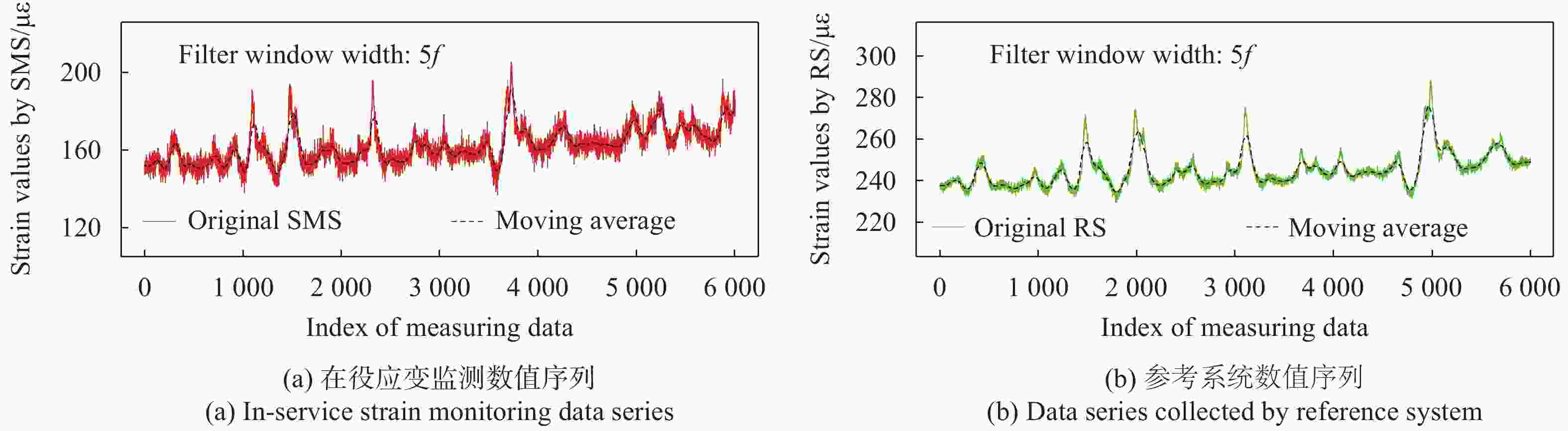
图 6 数据序列及预处理
Figure 6. Data series and preprocessing
由图6可知,两个数据序列不仅时间起止点和测值的分布区间不同,曲线形态的尺度也存在明显差异。依前述方法,对RS和SMS进行字符映射,步长与各系统的测量频率成正比,分别取40和30,映射字符集的字符总数
$t$ 取10。数值序列的匹配过程如图7所示。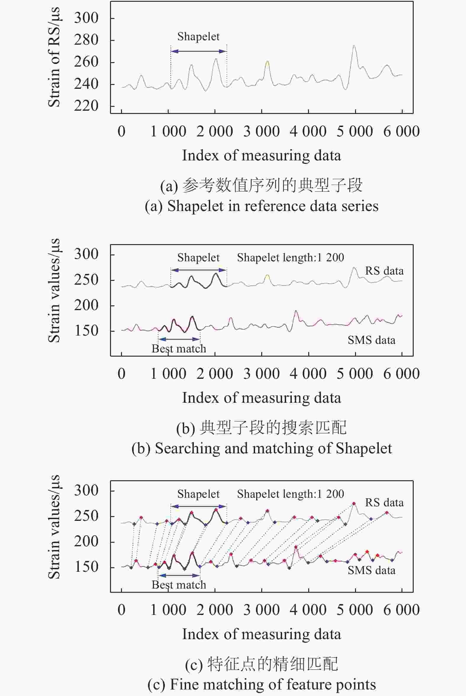
图 7 数据序列的匹配过程
Figure 7. Matching procedure of data series
如图7所示,在经预处理的RS数据序列中选取典型子段(Shapelet),其字符化表示为“abbddcbabehhfeddcaaabdhjjhecbb”;按照最小编辑距离原则,从SMS的字符化数据序列中搜索最佳初始匹配位置(图7(b));然后,以初始匹配位置为起点双向搜索,匹配峰值和谷值特征点(图7(c));最后,在相临特征点间进行精细化匹配,得到匹配测量值序列。
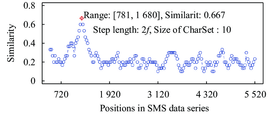
上述分析过程,在配置Intel(R) Core(TM) i7-3520M处理器的PC机上以R语言实现。不同位置匹配的相似度分布如图8所示。
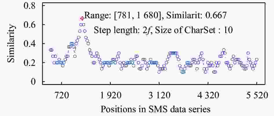
图 8 相似度及最佳匹配
Figure 8. Similarity and best match
-
对在役应变监测系统的性能评价是个抽样分析过程。由于数据采集过程是在不可控的被动激励源条件下完成的,无法通过人工干扰提升数据的代表性。该试验中,从连续两天的监测数据中抽取4段测值分布区间较宽的数据段进行分析。各数据段的样本数量、应变值的分布区间、序列形态,以及性能指标如表2所示。
表 2 取样数据段及系统性能指标计算
Table 2. Sampling data segment and system performance index calculation
Name Length/samples Range/µε Response curve ${C_{90}}$ ${C_{95}}$ ${C_{99}}$ Series A 50000 120.5-211.9 
0.0670 0.0805 0.1069 Series B 100000 115.5-211.9 
0.0638 0.0766 0.1018 Series C 50000 109.8-176.2 
0.0598 0.0719 0.0955 Series D 100000 102.3-176.2 
0.0559 0.0664 0.0877 表2中,
${C_{90}}$ 、${C_{95}}$ 和${C_{99}}$ 分别表示包含概率为90%、95%和99%时的性能指标。由于取样数据段的长度、测值区间、激励源条件的不同,最终评价指标的计算结果存在差异。但对于同一序列中不同长度的两段样本来说,其不同包含概率下的对应指标的差异不大。如序列A和B,其${C_{90}}$ 、${C_{95}}$ 和${C_{99}}$ 的差异均在0.006以内。对于序列C和D,其${C_{90}}$ 、${C_{95}}$ 和${C_{99}}$ 的差异在0.008以内。综上可知,文中所提方法对于评价在役应变监测系统的技术性能有一定的稳定性,但需考虑不同时段内激励条件的差异。
-
针对在役结构监测系统长期、连续使用中的计量性能在线评价难题,以光纤式结构应变监测系统的性能评价为目标,提出了基于数据序列特征分析的性能评价方法。该方法以参考系统建立数据动态比较的基准,通过自然激励条件下的匹配数据序列的结构特征分析,建立性能评价模型。针对数据分析评价过程中,不同形态尺度数据序列的匹配难题,提出了基于字符化表征的匹配方法。通过实际桥梁监测系统进行了现场试验验证,结果表明:
(1) 基于字符化表征和相似度的匹配方法,可适应不同测量频率、不同取样区间所导致的序列形态、尺度和位置差异条件下的数据序列匹配,有良好的适用性;
(2) 以匹配后数据序列的线性拟合残差的分布区间为基础,所建立的评价指标具有一定的稳定性,指标偏差不大于±1%,具有量化分析和演变追踪的实用性;
(3) 评价在役结构监测系统性能时,分析数据的取样过程宜适当考虑激励条件的影响。
Online evaluation method for the performance of in-service fiber optic strain monitoring systems
-
摘要: 结构监测系统的计量性能是结构安全状态评估的关键。针对在役结构监测系统长期、连续使用过程中的在线性能评价难题,依托光纤式结构应变监测系统的数据分析试验,提出了基于序列特征分析的结构监测系统性能评价方法。该方法以参考系统建立测量数据的动态比较基准,通过自然激励条件下的匹配数据序列的结构特征分析,建立性能评价模型。针对不同形态、尺度数据序列的匹配难题,提出了基于字符化表征的匹配方法。现场试验验证表明:该方法具备多尺度、大范围数据序列匹配的适应性,所提评价指标对于不同样本的计算偏差不大于±1%,具有监测系统长期量化评价的实用性。Abstract: The performance of the structural monitoring system (SMS) is the key of structural safety assessment. Aiming at the difficulties of evaluation for in-service SMS, an online performance evaluation method based on data series feature analysis was proposed. In this method, the reference system was used to establish the dynamic comparison benchmark of the measured data, and the performance evaluation model was established by analyzing the structure characteristics of the matched data series under the natural excitation condition. A method based on character representation was proposed to solve the matching problem of data series of different shapes and scales. The field tests show that this method has the adaptability of multi-scale and large-range data series matching, and the calculation deviation of the proposed evaluation indexes for different samples is less than ±1%, so it has the practicability of long-term quantitative evaluation of the structural monitoring systems.
-
表 1 光纤应变传感器参数
Table 1. Parameters of the fiber strain sensors
SN Stain coeff./
µε·nm−1Temperature coeff./
µε·nm−1Init. wavelength/
nm#669 778.0437 −789.5004 1553.151 #592 726.0287 −669.8661 1545.491  下载: 导出CSV
表 2 取样数据段及系统性能指标计算
Table 2. Sampling data segment and system performance index calculation
Name Length/samples Range/µε Response curve ${C_{90}}$ ${C_{95}}$ ${C_{99}}$ Series A 50000 120.5-211.9 0.0670 0.0805 0.1069 Series B 100000 115.5-211.9 0.0638 0.0766 0.1018 Series C 50000 109.8-176.2 0.0598 0.0719 0.0955 Series D 100000 102.3-176.2 0.0559 0.0664 0.0877
下载: 导出CSV
-
[1] Annamdas Venu Gopal Madhav, Bhalla Suresh, Soh Chee Kiong. Applications of structural health monitoring technology in Asia [J]. Structural Health Monitoring, 2017, 16(3): 324-346. doi: 10.1177/1475921716653278 [2] Wang Longbao, Mao Yingchi, Cheng Yangkun, et al. Deep learning-based diagnosing structural behavior in dam safety monitoring system [J]. Sensors, 2021, 21(4): 1171. doi: 10.3390/s21041171 [3] Liu Yang, Li Hu, Wang Yongliang, et al. Damage detection of tunnel based on the high-density cross-sectional curvature obtained using strain data from BOTDA sensors [J]. Mechanical Systems and Signal Processing, 2021, 158: 107728. doi: 10.1016/j.ymssp.2021.107728 [4] Tochaei Emad Norouzzadeh, Fang Zheng, Taylor Todd, et al. Structural monitoring and remaining fatigue life estimation of typical welded crack details in the Manhattan Bridge [J]. Engineering Structures, 2021, 231: 111760. doi: 10.1016/j.engstruct.2020.111760 [5] Seo Junwon, Hu Jong Wan, Lee Jaeha. Summary review of structural health monitoring applications for highway bridges [J]. Journal of Performance of Constructed Facilities, 2016, 30(4): 4015072. doi: 10.1061/(ASCE)CF.1943-5509.0000824 [6] Bado Mattia Francesco, Casas Joan R. A review of recent distributed optical fiber sensors applications for civil engineering structural health monitoring [J]. Sensors, 2021, 21(5): 1818. doi: 10.3390/s21051818 [7] Zhang Kaiyu, Yan Guang, Meng Fanyong, et al. Temperature decoupling and high strain sensitivity fiber Bragg grating sensor [J]. Optics and Precision Engineering, 2018, 26(6): 1330-1337. (in Chinese) doi: 10.3788/OPE.20182606.1330 [8] Wang Huaping, Xiang Ping. Optimization design of optical fiber sensors based on strain transfer theory [J]. Optics and Precision Engineering, 2016, 24(06): 1233-1241. (in Chinese) doi: 10.3788/OPE.20162406.1233 [9] Lv Anqiang, Li Yongqian, Li Jing, et al. Distinguish measurement of temperature and strain of laid sensing optical fibers based on BOTDR [J]. Infrared and Laser Engineering, 2015, 44(10): 2952-2958. (in Chinese) [10] Li Lili, Liu Gang, Zhang Liangliang, et al. Sensor fault detection with generalized likelihood ratio and correlation coefficient for bridge SHM [J]. Journal of Sound and Vibration, 2019, 442: 445-458. doi: 10.1016/j.jsv.2018.10.062 [11] Peng Lu, Jing Genqiang, Luo Zhu, et al. Dynamic strain signal monitoring and calibration with neural network based on hierarchical orthogonal artificial bee colony [J]. Computer Communications, 2020, 159: 279-288. doi: 10.1016/j.comcom.2020.05.028 [12] Jing Genqiang, Yuan Xin, Duan Fajie, et al. Matching method for data sequences from on-line calibration of laser displacement meter [J]. Infrared and Laser Engineering, 2019, 48(5): 0506006. (in Chinese) [13] Lin Jessica, Keogh Eamonn, Wei Li, et al. Experiencing SAX: A novel symbolic representation of time series [J]. Data Mining and Knowledge Discovery, 2007, 15(2): 107-144. doi: 10.1007/s10618-007-0064-z [14] Ye Lexiang, Keogh Eamonn. Time series shapelets: A novel technique that allows accurate, interpretable and fast classification [J]. Data Mining and Knowledge Discovery, 2011, 22(1-2): 149-182. doi: 10.1007/s10618-010-0179-5 -

 点击查看大图
图(8) / 表(2)
计量
- 文章访问数: 217
- HTML全文浏览量: 63
- PDF下载量: 27
- 被引次数: 0


