


-
2012年,成功在盖尔撞击坑(Gale Crater)上着陆的“火星科学实验室”(Mars Science Laboratory,MSL)所释放的好奇号火星车携带了ChemCam激光诱导击穿光谱仪等数台先进复杂的科学仪器。其中,搭载的ChemCam激光诱导击穿光谱仪器已经获得了超过60万份来自火星表面的LIBS光谱,覆盖了近1000个不同的岩石和土壤目标,用来精确分析不同目标的样品的元素成分与光谱特征。其面临的主要挑战之一是如何克服基体效应,得到准确的定量结果。激光诱导击穿光谱 (Laser Induced Breakdown Spectroscopy,LIBS)是一种快速化学分析技术,它使用短激光脉冲在样品表面产生微等离子体。基于火星表面探测环境的特殊性,激光诱导击穿光谱技术对比其他光谱技术具有可实现远程探测、分析高效快速、可剥离岩石表面灰尘、有广泛的元素覆盖范围(包括较轻的元素,例如 H、Be、Li、C、N、O、Na 和 Mg)、包含多功能采样协议等独特的优势,成为太空探测中具有巨大优势的一种先进技术[1]。LIBS 技术对于元素的定量检测研究多集中于谱线强度的辨识与统计分析上,仍有较大的挖掘空间,由于光谱数据矩阵复杂、在高维空间自变量之间相关性较大,因此需要提取有用的特征光谱信息,减小计算机运算量,并建立可靠而稳定的模型,达到预测的精度。
传统的激光诱导击穿光谱光谱分析主要使用多变量分析方法,且对行星地质领域LIBS分析较少。付林等通过激光诱导击穿光谱技术在空气和低气压条件下分别对RDX和TNT两种有机爆炸物进行检测,发现CN (421.3 nm)和C2(516.2 nm)是有机爆炸物最有研究价值的两条谱线[2]。杨彦伟等基于外加腔体约束方法,对铝土矿中Al、Si两种元素的激光诱导击穿光谱实验参数进行了优化研究[3]。任佳等采用了飞秒激光成丝-纳秒脉冲激光诱导击穿光谱技术(Filamentns DP-LIBS)对土壤中重金属铅元素进行了定量分析[4]。陈世和等用激光诱导击穿光谱法直接检测煤粉流时对主要控制因素进行优化,并采用正交实验法考察了3个主要控制因素对激光诱导击穿光谱测量煤粉流的影响[5]。李晨毓等采用激光诱导击穿光谱结合激光共聚焦显微镜,对河南省上蔡郭庄楚国墓葬群出土的青铜器和故宫博物院灵沼轩的陶瓷砖成分进行表面及深度分布分析[6]。李昂泽等基于激光诱导击穿光谱技术,采集了不同种类烟草的原子发射光谱,并结合支持向量机方法,实现了烟草的快速分类鉴别[7]。杨友良等使用了粒子群方法(Particle Swarm Optimization, PSO)优化支持向量回归方法(Support Vector Regression, SVR)的参数用以分析 LIBS 光谱,预测钢液中的多种元素含量,获得了较普通支持向量回归方法更好的准确度[8]。Anderson 等按照对应目标成分的浓度将 LIBS 光谱划分为数个子集,再使用偏最小二乘回归方法(Partial Least Squares Regression, PLSR)分别进行分析,获得了较单独的 PLSR 分析更好的结果[9]。Clegg 等结合了偏最小二乘方法(Partial Least Squares, PLS)和独立主成分分析方法(Independent Component Analysis, ICA),进行对 LIBS 光谱的分析,进一步提高了激光诱导击穿光谱定量建模的准确度[10]。同样,由于深度学习领域的不断进步,其不断在多元复杂耦合问题分析上展现出优势,不少学者也开始尝试使用深度学习方法分析光谱数据。马翠红等使用遗传神经网络(Genetic Neural Network, GNN)结合 LIBS 定量预测钢液中锰元素,取得了较为准确的结果[11]。浙江大学的林涛团队基于深度学习方法,设计了DeepSpectra 模型,用于分析农产品产生的 LIBS 光谱,也有效改善了预测准确度[12]。
基于光谱数据的高维度特征性,笔者将光谱数据按照三通道折叠为三层特征图,作为ResNet网络的输入,从而预测校准标样中包含的Si、Ti、Al、Fe、Mg、Ca、Na、K等主元素含量。由于光谱数据属于原一维特征数据,所以相关研究大多使用1D卷积来处理数据,这样对基体效应消除效果有限。2D卷积可以让不同波长的谱线之间有机会被一起扫描分析,可以更有效地减弱基体效应的影响。另一方面,随着网络结构的加深,一些问题也就随之产生,例如梯度弥散和梯度爆炸。这两种问题都是由于神经网络的特殊结构和特殊求参数方法造成的,也就是链式求导的间接产物[13]。文中引入了残差网络进行光谱数据的特征信息的提取,使信息更容易在各层之间流动,包括在前向传播时提供特征重用,在反向传播时缓解梯度信号消失,最终获得的实验结果误差较传统定量分析方法线性支持向量机回归LinearSVR和深度可分离卷积网络Xception有显著改善。
-
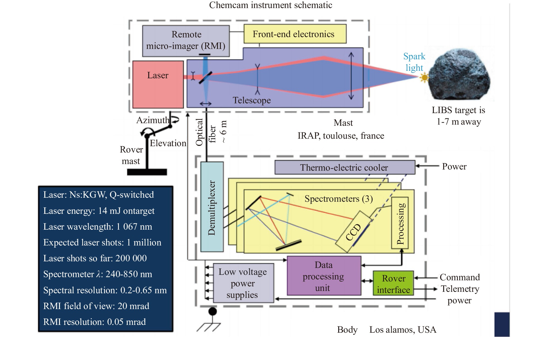
ChemCam 是 2012 年美国发射登陆火星的好奇号(Curiosity)上所携带的 LIBS设备,其也是第一台用于行星探索的 LIBS 设备。文中使用的 LIBS 光谱数据均来自美国国家航空航天局行星数据系统(National Aeronautics and Space Administration Planetary Data System, NASA PDS),其使用ChemCam及其备份样机制备数据。ChemCam 中具有三台 2 048 通道的光谱仪,分别覆盖波长范围 240.1~342.2 nm,382.1~469.3 nm,474.0~906.5 nm。其使用波长为1067 nm的 Nd∶KGW激光,设置 350 μm 光斑尺寸,5 ns 激光脉冲宽度,14 mJ 脉冲能量。设备整体被放置于 933 Pa 二氧化碳环境下用于模仿火星大气环境。采集时样品被放置在1.5 m远处,ChemCam 将在样品上五处不同的位置各发射 50 次激光脉冲并记录,具体过程如图1所示。最终每种样品记录约 250 条光谱,每条光谱具有240.1~906.5 nm 中的6 144个通道。
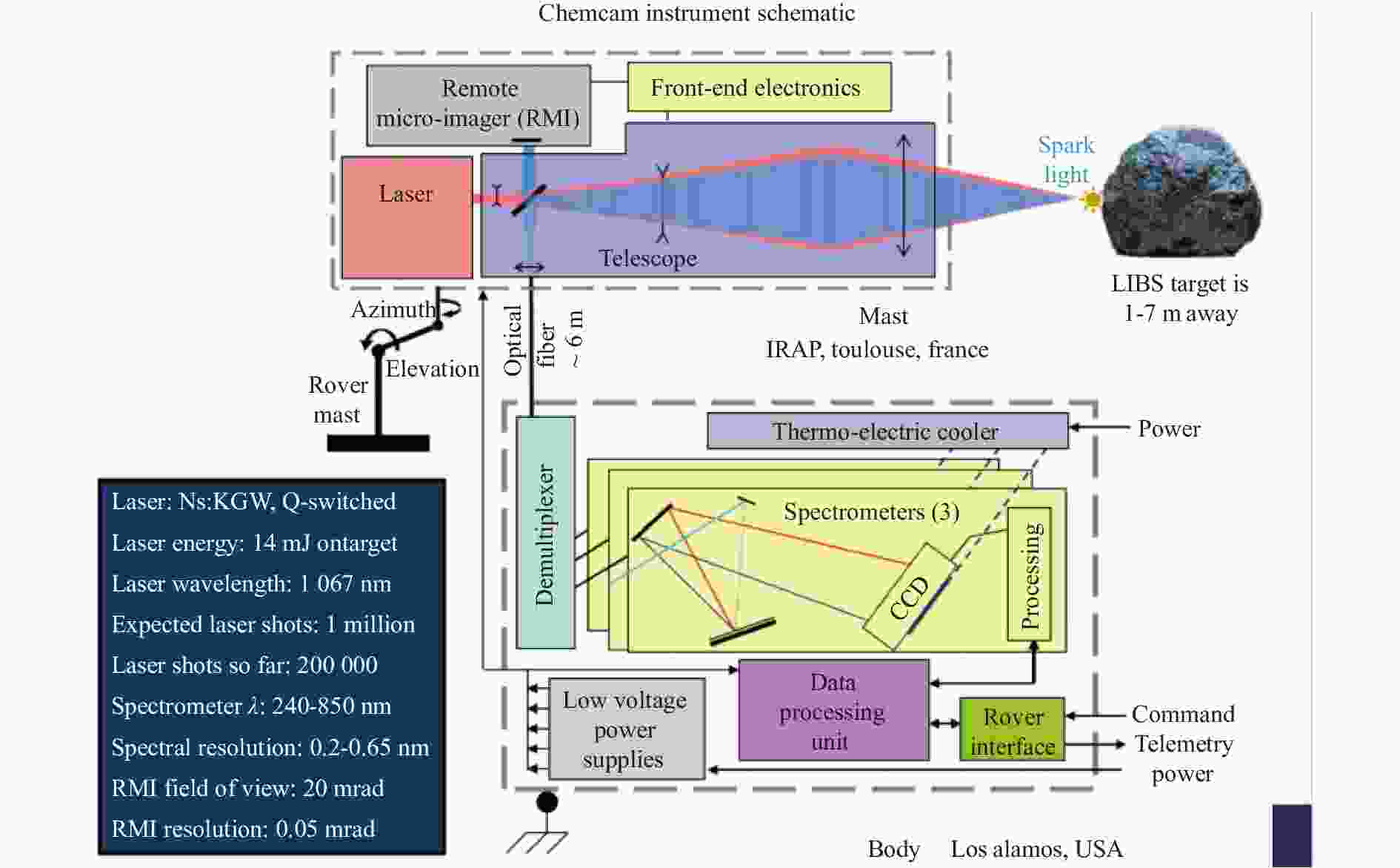
图 1 ChemCham设备工作原理示意图
Figure 1. Principle diagram of ChemCham equipment working
ChemCam 校准数据库包括了 408 个化学成分独立测量的压制粉末样品。用标准地质化学方法测定了各个实验样品的8种主要成分组成(包括SiO2、TiO2、Al2O3、FeOT(包括铁单质及铁氧化物)、MgO、CaO、Na2O、K2O)。在被激光产生的冲击波清除之前,通常会在一定程度上有来自覆盖在目标上的灰尘的污染,并不用于确定目标的元素组成,所以丢弃前5次激光聚焦照射的采集得到的等离子体光谱。然后将每个位置的后续 45 个等离子光谱平均,得出每个样品 5 个光谱(总共 2 040 个光谱)。这些实验样品由纽约州立大学石溪分校的 McLennan 实验室、NASA Johnson 航天中心的 Morris 实验室、Mount Holyoke College 的 Dyar 实验室以及加州理工学院的 Ehlmann 实验室提供。McLennan 实验室提供的样品是来自各种地质环境的沉积岩和准沉积岩。Morris 实验室样品是多种矿物和岩石,已用于校准火星探测漫游者(Mars Exploration Rover, MER)、火星凤凰号着陆器(Mars Phoenix Lander)和火星科学实验室上的多种仪器。Dyar 实验室的样品是火成岩和含硫酸盐的岩石,而 Ehlmann 实验室的样品则是一套经过改变和未改变的铁镁质火山岩样品,以及盐和氧化物与玄武岩的混合物。
文中使用的 408 个实验样品对应的等离子体光谱分别保存在实验样品对应名称文件夹内,每个文件夹包括 5 个 CSV(Comma-Separated Values)文件,对应于5个激光聚焦点的等离子体光谱数据,每个 CSV 文件中保存有对应激光聚焦点照射 50 次生成的 50 组光谱数据和这些光谱数据的平均值与中位数。同时还有一个 CSV 文件保存有每个实验样品对应的名称与主要成分的含量。
图2 为 样本中8 种主成分目标元素含量示意图。
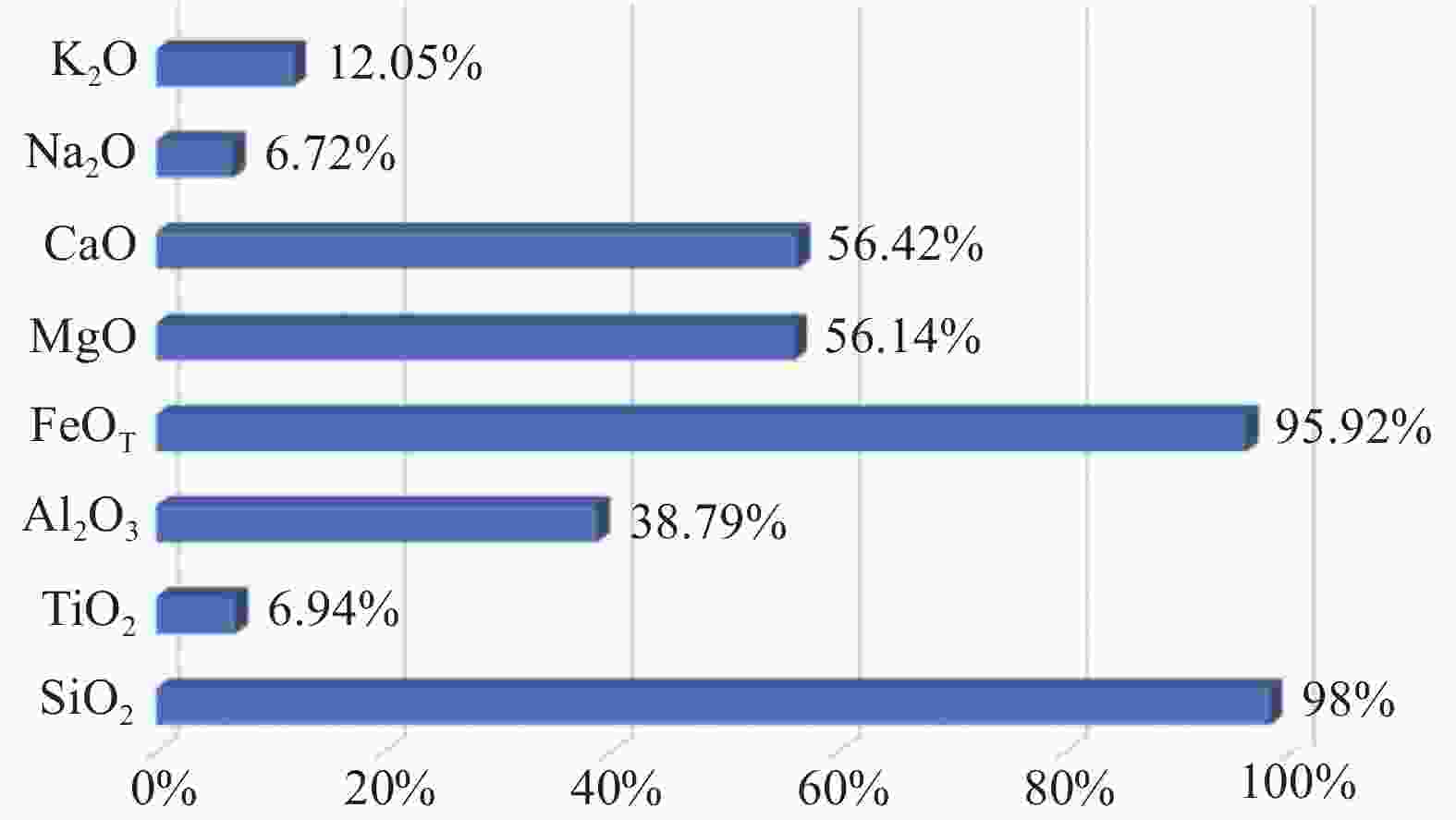
图 2 样品中主要成分丰度范围
Figure 2. Abundance range of main components in the sample
-
限制LIBS用于定量检测的重要因素之一是基体效应, 引起基体效应的原因是样品的物理和化学性质差异, 以及激光与物质相互作用的非线性, 这种非线性导致在激光烧蚀、 等离子体产生、 膨胀等过程中电子温度、 电子密度和烧蚀量等受到影响[14]。 因此, 基体效应的研究对LIBS定量分析中有重要的意义[15]。
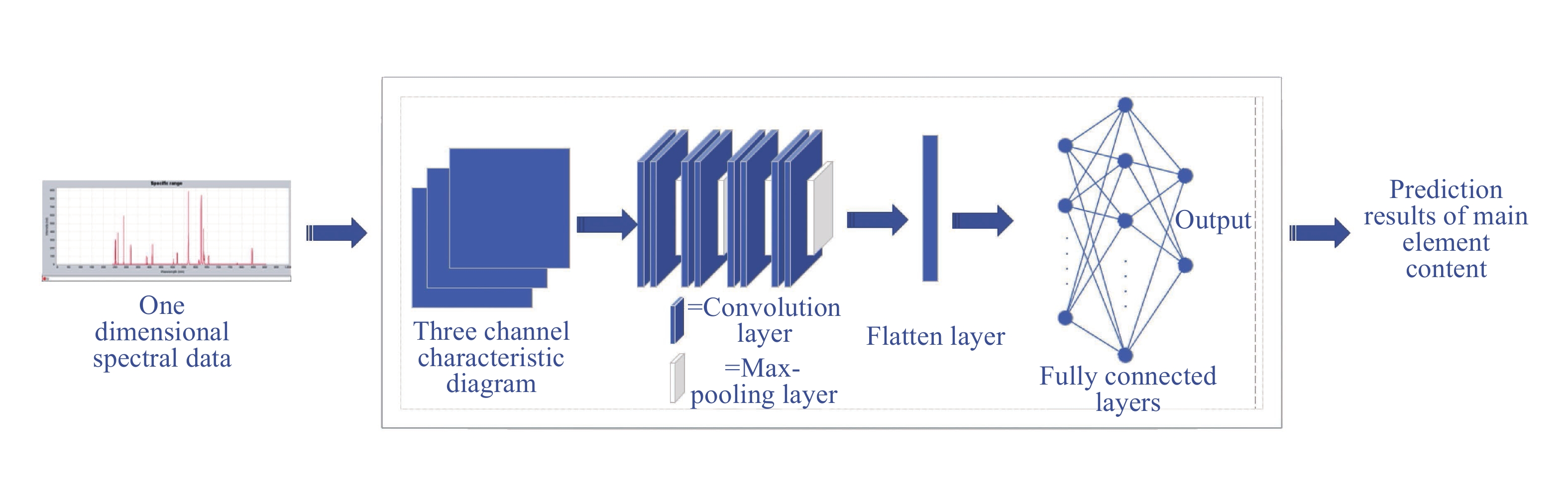
基于光谱数据本身的高维度复杂性,如果将其视为一维数据用1D卷积核进行卷积处理,往往由于不能整体性考虑数据间的基体效应而产生预测结果之间的误差。故而文中将6144通道的光谱数据提取出其中的6075D光谱信息进行折叠并正态分布归一化,将其转变为45×45×3的三通道特征图投入ResNet网络结构进行训练,使不同波段之间的数据可以同时参与2D卷积运算,极大地降低了模型本身的复杂度,且在一定程度上减弱了基体效应对定量分析的影响。图3是将光谱数据三通道折叠并进行卷积运算输出预测结果的示意图。
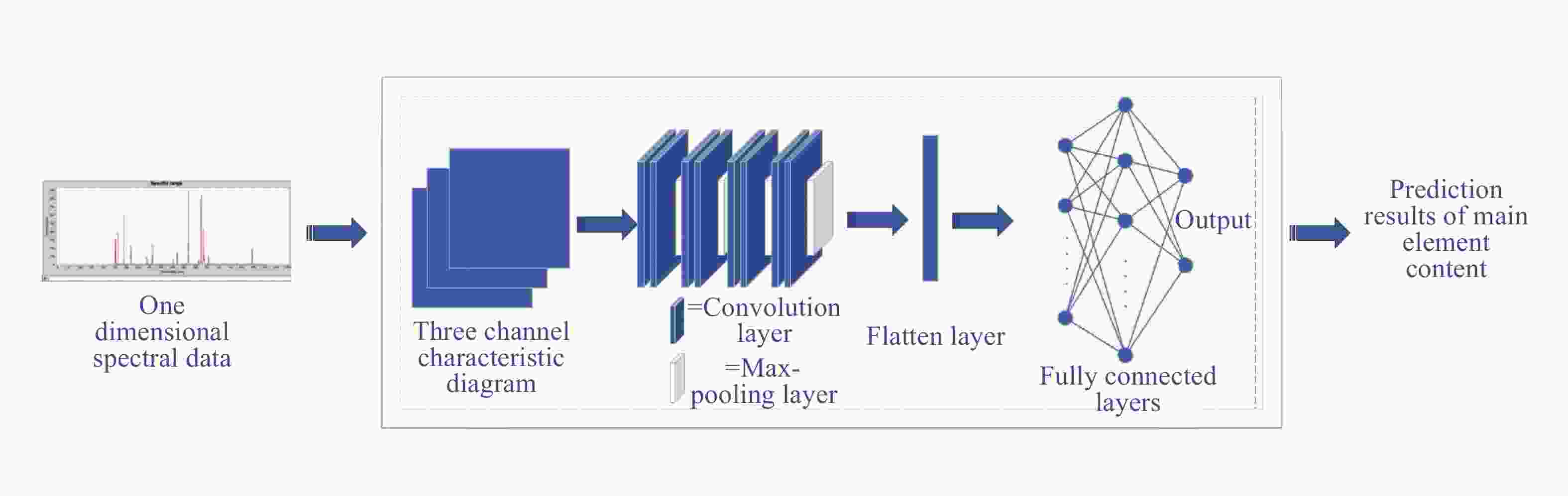
图 3 光谱数据三通道折叠并进行卷积运算示意图
Figure 3. Schematic diagram of three channel folding and convolution operation of spectral data
-
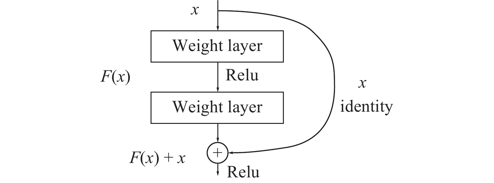
卷积神经网络(Convolutional Neural Network, CNN)通常在高维数据特征维度提取方面特别是在处理图像信息等多通道高维数据时相对于传统方法有显著提升。文中引入了深度残差网络学习框架来对光谱数据进行处理,相比于让一些堆叠层直接学习原始特征,而是让堆叠层去拟合残差映射(即恒等映射变换),从而解决了深度学习模型堆叠产生的退化问题。图4是ResNet[16]中的核心结构:残差块Residual block的示意图。

图 4 ResNet残差连接块
Figure 4. ResNet residual connection block
图4中右侧的曲线是跳接(Shortcut Connection),通过跳接在激活函数前,将上一层(或几层)之前的输出与本层计算的输出相加,将求和的结果输入到激活函数中做为本层的输出。用数学语言描述,假设Residual Block的输入为
$ x $ ,则输出$ y $ 等于:$$ y = F(x,\{ {W_i}\} ) + x $$ (1) 式中:
$ F(x,\{ {W_i}\} ) $ 为优化求解的目标。以上图为例,残差部分是中间有一个Relu激活的双层权重,即:$$ F = {W_2}\sigma ({W_1}x) $$ (2) 式中:
$ \sigma $ 指代Relu激活函数;$ {W_1},{W_2} $ 指代两层权重。由于引入了跳跃连接,这可以使上一个残差块的信息没有阻碍地流入到下一个残差块,提高了信息流通,并且也避免了由于网络结构过深所引起的梯度消失问题和退化问题。 -
ResNet-152是一个具有152层的残差网络,在这项研究中,要分析的是从光谱数据中折叠产生的三通道特征图,这些数据与ImageNet中的用于预训练权重的图像数据有很大的不同。因此,需要对预训练的ResNet-152网络的后2层,即完全连接层、Softmax分类层进行修改。将全连接层去除,以防止训练中模型参数量的快速增长,从而使训练的模型更加轻便。又因为研究主要解决的是主元素含量预测的回归问题,所以将Softmax分类子层改为了Linear线性整流层,使其更适用于校准标样的主元素含量预测。最后将修改后的ResNet-152网络重新训练以产生新的参数,表1所示为改进后用于预测标样的主元素含量的ResNet152网络。
表 1 用于预测的改进ResNet152 网络结构参数配置
Table 1. Improved ResNet152 network structure confi-guration parameters for prediction
Layer name Output size ResNet152 Feature maps Convolution 112×112 77 conv, 64, stride2 64 Pooling 56×56 3 × 3 max pool, stride2 64 Residul block(1) 56×56 1 × 1,64 256 3 × 3, 64 × 3 1 × 1, 256 Residul block(2) 28×28 1 × 1, 128 512 3 × 3, 128 × 8 1 × 1, 512 Residul block(3) 14×14 1 × 1, 256 1024 3 × 3, 256 × 36 1 × 1, 1024 Residul block(4) 7×7 1 × 1, 512 2 048 3 × 3, 512 × 3 1 × 1, 2048 Linear layer 1×1 Linear 采用上述的ResNet-152网络结构来进行光谱数据的特征提取时,输出层之前加入了Dropout[17]机制来防止由于网络结构过深而在训练时产生的过拟合现象。这样可以让模型的泛化性更强,使其不会太依赖训练数据的某些局部的特征,这也对光谱数据起到了一定的降噪滤波作用,从而使预测误差进一步降低。
-
为了评估网络模型训练和测试过程的准确度,需要在ResNet152网络模型训练时加入度量函数。决定系数R2(Coefficient of Determination)常常在线性回归中被用来表征有多少百分比的因变量波动被回归线描述。R2越趋近于1,则模型的预测准确率越高。R2定义表达式如下[18]:
$$ {R^2}{\text{ = }}{\rm SSR}/{\rm SST} = 1 - {\rm SSE}/{\rm SST} $$ (3) 式中:SST=SSR+SSE;SST(Total Sum of Squares)为总平方和;SSR(Regression Sum of Squares)为回归平方和;SSE(Error Sum of Squares) 为残差平方和。将R2分数引入到模型的编译中,能在训练时同时针对预测含量Loss值均方根误差RMSE(Root Mean Square Error)和预测准确率进行优化,从而提高模型表现。
为了提高模型精度,文中研究设置了模型每迭代10次学习率指数衰减为原来的1/2,使模型逐渐逼近误差最小值。若学习率较大,在算法优化的前期会加速学习,但是在后期会有较大波动,甚至出现损失函数的值围绕最小值徘徊,模型难以收敛达到最优的情况。以指数衰减方式进行学习率的更新简单直接,收敛速度快,可以使ResNet152网络模型在训练时达到更高的预测精度。衰减的学习率的大小和训练次数呈指数相关,其更新规则为[19]:
$$ r = {r_0}× d_r^{\tfrac{{{p_1}}}{{{p_2}}}} $$ (4) 式中:
$ {p_1} $ 为计数器, 从0计数到训练截止时的迭代次数;$ {r_0} $ 为初始化的学习率;dr为衰减速率;学习率 r 随着$ {p_1} $ 的递增而衰减;$ {p_2} $ 用于控制指数衰减速度。 -
该实验从ChemCam 校准数据库的 408个实验样品对应的等离子体光谱中随机抽取样本数据,按照8:1:1的比率划分训练集、验证集和测试集。训练集用来训练模型,验证集用来检验模型精度并调参,测试集用来验证模型在未知数据上的预测表现。文中选取了不同标样划分数据集,测试集中标样数据未出现在训练集中,可充分检测模型泛化能力。
为了验证ResNet-152网络结构在处理高维度光谱数据时的表现,选取了线性支持向量机回归LinearSVR(Linear Support Vector Machine Regression)和深度学习领域InceptionV3网络的改进版本,一种完全基于深度可分离卷积层的卷积神经网络体系结构Xception[20]作为对比。自从首次推出以来,Inception系列网络一直是ImageNet数据集以及Google使用的内部数据集(尤其是JFT)上性能最好的模型系列之一。Depthwise Separable Convolution是对每一个通道执行空间卷积,保证通道特征的分离,再对整体进行深度卷积。随着要提取的属性越来越多,深度可分离卷积可以节省更多的参数,如图5所示。
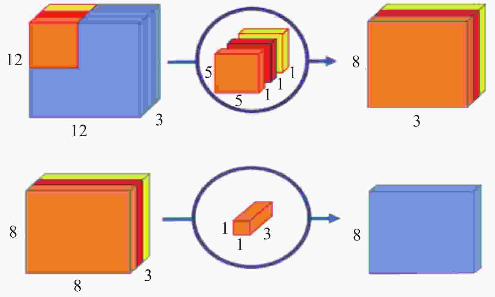
图 5 对每一个通道执行空间卷积后对整体进行深度卷积
Figure 5. Deep convolution of the whole after spatial convolution for each channel
如图6所示,Xception则将上述Depthwise Separable Convolution模型操作的顺序颠倒,先通过1×1卷积进行所有通道的特征提取,再对提取出的矩阵每一个(或几个)通道进行单独的卷积,将每一块通道输出连接成最终输出向量,从而得到更精确的预测结果。

图 6 一个简化的Xception模型
Figure 6. A simplified Xception model
文中选择了两种评估指标,均方根误差(Root Mean Squared Error,RMSE)和决定系数R2(coefficient of determination)来评测模型预测表现。RMSE的具体计算表达式如下:
$$ RMSE = \sqrt {\frac{1}{m}\sum\nolimits_{i = 1}^m {{{(y_{test}^{(i)} - \hat y_{test}^{(i)})}^2}} } $$ (5) 针对标样元素含量预测,RMSE和MAE(Mean Absolute Error)有一定局限性:同一个算法模型,预测不同元素的含量,不能体现此模型针对不同含量预测所表现的优劣。不同实际应用中,数据的量纲不同,无法直接比较预测值,因此无法判断模型更适合预测哪个问题。所以文中在神经网络训练时加入R2分数,从而将预测结果转换为准确度,将比较标准规约到[0, 1]之间,便于比较模型预测效果。
针对统一元素含量值预测度量时,RMSE代表着预测值和真实值之间的偏差,RMSE越接近0,则预测值和真实值之间误差越小,而
$ {R^2} $ 越接近1,则表示预测值更接近真实值。实验得到的结果如表2所示。表 2 元素含量预测值RMSE和R2分数对比
Table 2. Comparison of RMSE and R2 scores of element content prediction values
LinearSVR Xception ResNet152 Element RMSE R2 RMSE R2 RMSE R2 SiO2 5.28 0.78 4.48 0.84 3.69 0.89 TiO2 0.62 0.39 0.51 0.57 0.59 0.42 Al2O3 3.77 0.52 3.68 0.54 3.36 0.62 FeOT 2.53 0.74 2.34 0.85 2.25 0.86 MgO 1.66 0.86 1.26 0.92 1.04 0.94 CaO 1.99 0.95 1.45 0.97 1.01 0.99 Na2O 0.68 0.75 0.63 0.81 0.61 0.83 K2O 0.74 0.76 0.46 0.91 0.43 0.95 由上表可知,相较于LinearSVR与Xception,ResNet在预测元素含量值时通常有着相对更低的RMSE和更高的
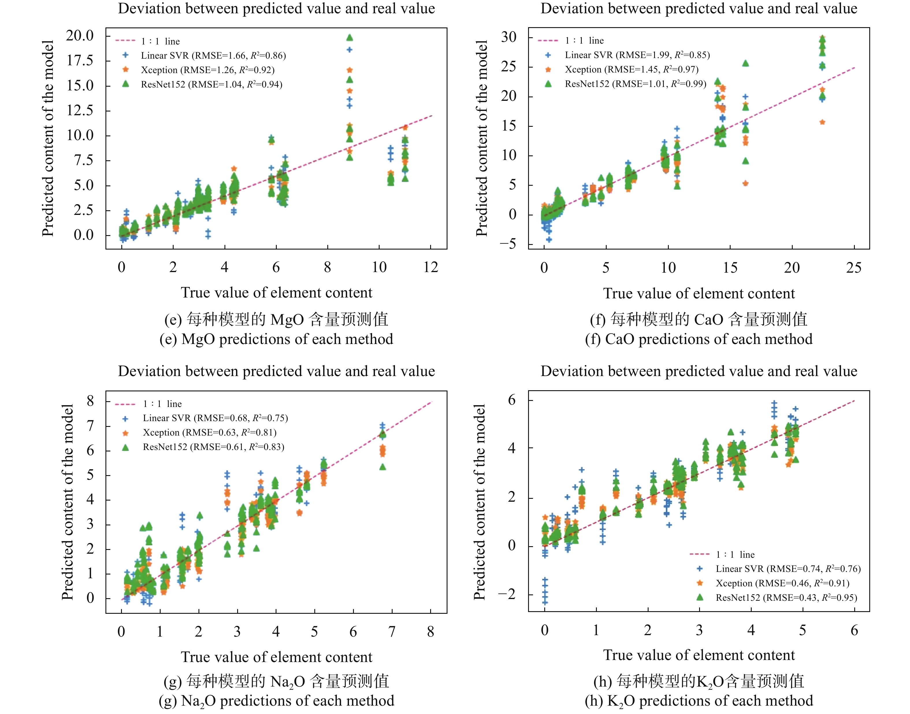
$ {R^2} $ 值,除了TiO2之外,ResNet相对于LinearSVR和Xception都有着更高的预测准确度。图7(a)~(h)是针对每种具体的主量元素含量值的预测结果和评价标准做可视化展示。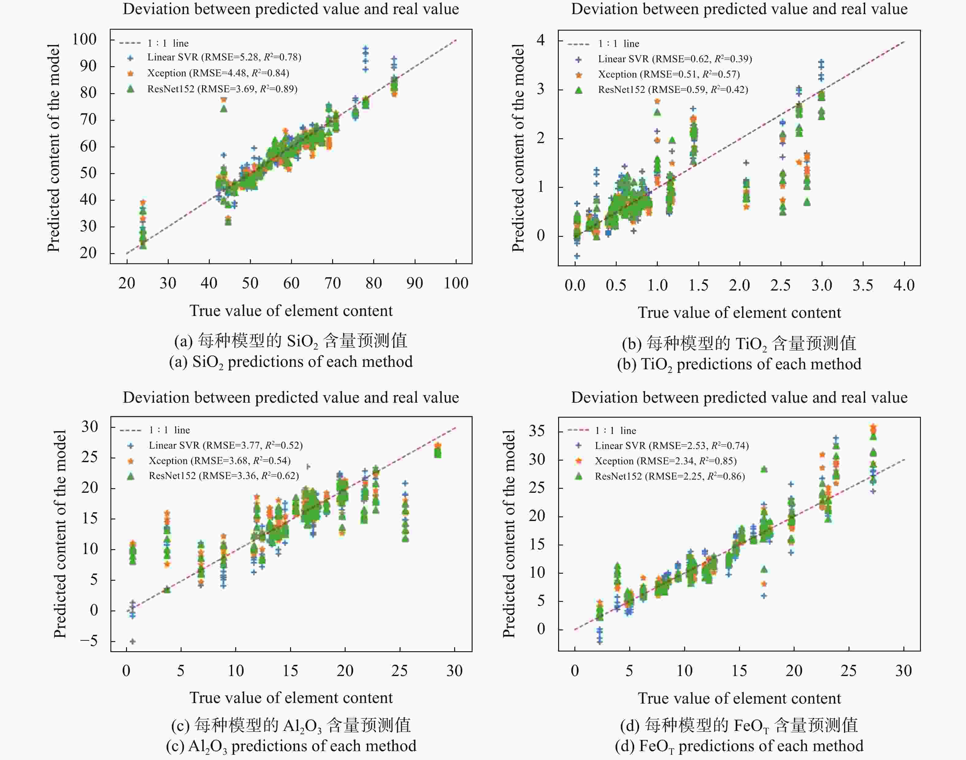
由文中的可视化结果可以看出,相较于其他元素,Si和Fe元素的预测值结果点更集中在1∶1线附近。对于Ti元素,在元素含量真实值大于2.0时,模型预测结果普遍低于真实值,而元素含量小于2.0的预测值较接近真实值。可能是由于样本中Ti的含量较少且离群值较多,导致预测误差偏大。故而可以针对Ti元素设置阈值2.0,针对阈值两侧的光谱数据分别建模。但是对于Al元素来说,含量范围处于10~20区间内的数据预测值较为接近真实值,而其他含量的预测值偏离较大,可以对其他含量区间的元素采用与原模型不同的学习率训练,会达到更好的效果。针对Mg元素,可以看到在含量值为9附近预测值误差较大,这极有可能是样本中存在部分异常值,可以针对性的对数据进行清洗或者归一化处理,从而改善模型含量值的预测表现。

图 7 各模型对应的各主成分含量预测值
Figure 7. Predicted content of each principal component corresponding to the models
从上述结果可以看出,ResNet-152模型的预测表现仍要普遍优于Xception和LinearSVR,体现在图中就是绿色的预测点相对更集中,均方根误差更小且R2分数更接近1。针对于个别含量值预测偏差较大的情况,可能是因为网络中的最大池化层用最大值代替原数据,造成了原光谱数据的特征模糊,进而导致网络修正参数能力下降。池化相当于在空间范围内做了维度约减,从而使模型可以抽取更加广范围的特征。同时减小了下一层的输入大小,进而减少计算量和参数个数,但同时也舍弃了原来数据中的细微特征值。针对该问题,笔者将在后续工作中改进网络结构,针对不同的元素含量值设定不同的池化操作,使之更适用于光谱数据的定量分析与建模。
此外,由于样本中光谱数据对应的元素含量值存在Nan(Not a Number)值,笔者的普遍处理是把其赋予样本元素含量的平均值,这样处理并没有考虑到对应光谱本身的特征,相信后续对其赋值方法改进后会使算法有更进一步的表现。同时对于样本中的离群值笔者并未进行处理,这会使它们的预测结果产生较大偏离从而拉高RMSE值。下一步工作可以将这些离群值和对应的光谱数据单独提取出来训练,或者划分出不同的含量区间进一步细分化建立模型,从而针对不同光谱波段对应不同元素含量的预测结果做出优化。
-
文中首先介绍了对 LIBS 光谱进行定量分析的背景和意义,简述了目前国内外使用多元线性回归或深度学习等方法分析 LIBS 光谱的研究现状。在此基础上,文中介绍了ChemCam 设备的原理,讲解了文中使用的数据的产生环境,描述了文中数据的划分方法及依据。之后,文中简述了深度学习方法的原理,提出使用ResNet模型用做光谱分析,解释了模型结构构成和模型中的优化机制。最后,文中对模型进行仿真,对比实验结果于 LinearSVR 和 Xception 模型,分析结果并探究了 LIBS 光谱分析和深度学习方法的特点。实验结果表明,通过对光谱数据进行三通道折叠后投入残差网络ResNet进行训练来预测元素含量值,不需要对光谱信息进行降维处理,极大地保留了原来光谱的高维度特征信息,从而降低了元素对应预测误差。此外ResNet相较于传统的LinearSVR(线性支撑向量机回归)方法和深度可分离卷积Xception网络,预测光谱数据对应的元素含量值时有更小的RMSE误差和更高的R2分数,体现出了更好的模型预测效果。
Quantitative analysis research of ChemCam-LIBS spectral data of Curiosity rover
-
摘要: 传统的偏最小二乘法和支持向量机回归等方法在预测光谱对应的火星车地面标样成分元素含量时往往难以获得较高的精度,并难于进一步优化。针对上述问题,在研究中对高维度光谱信息进行三通道折叠以消除其基体效应,并引入在计算机视觉领域表现不俗的ResNet残差网络结构来提取光谱特征并预测对应主成分含量值。文中将ResNet网络结构中的全连接层去除以避免模型参数快速增长,并将网络最后的Softmax分类子层改为线性整流层以便于进行预测,同时添加了指数学习率衰减和Dropout机制以使模型预测结果具备更高的精度与泛化能力。模型各主要元素含量的预测均方根误差相对于线性支持向量机LinearSVR和深度可分离卷积网络Xception分别平均下降了30%和17%。实验结果表明:采用LIBS技术对ChemCam光谱数据进行主成分元素定量分析时,基于ResNet网络建立的回归模型表现出良好的预测特性。Abstract: The traditional partial least squares method and support vector machine regression method were often difficult to obtain high accuracy and further optimization in predicting the element content of the ground standard sample of the rover corresponding to the spectrum. To solve the above problems, the three-channel folding of high-dimensional spectral information was carried out to eliminate its matrix effect in the research, and introduced the Residual Network structure (ResNet), which was good in the field of computer vision, to extract the spectral features and predict the corresponding principal component content. In this paper, the full connection layer in ResNET network structure was removed to prevent the sudden increase of model parameters, and the last Softmax classification sublayer of the network was changed into a linear rectification layer for prediction. At the same time, exponential learning rate attenuation and Dropout mechanism were added to make the model prediction results have higher accuracy and generalization ability. Compared with linear support vector machine regression (LinearSVR) and depth separable convolution network Xception, the prediction root mean square error of each main element content of the model decreases by 30% and 17% on average, respectively. The experimental results show that the regression model established by ResNet network shows good prediction characteristics when LIBS technology is used for principal element quantitative analysis of ChemCam spectral data.
-
图 3 光谱数据三通道折叠并进行卷积运算示意图
Figure 3. Schematic diagram of three channel folding and convolution operation of spectral data
图 5 对每一个通道执行空间卷积后对整体进行深度卷积
Figure 5. Deep convolution of the whole after spatial convolution for each channel
7 各模型对应的各主成分含量预测值
7. Predicted content of each principal component corresponding to the models
表 1 用于预测的改进ResNet152 网络结构参数配置
Table 1. Improved ResNet152 network structure confi-guration parameters for prediction
Layer name Output size ResNet152 Feature maps Convolution 112×112 77 conv, 64, stride2 64 Pooling 56×56 3 × 3 max pool, stride2 64 Residul block(1) 56×56 1 × 1,64 256 3 × 3, 64 × 3 1 × 1, 256 Residul block(2) 28×28 1 × 1, 128 512 3 × 3, 128 × 8 1 × 1, 512 Residul block(3) 14×14 1 × 1, 256 1024 3 × 3, 256 × 36 1 × 1, 1024 Residul block(4) 7×7 1 × 1, 512 2 048 3 × 3, 512 × 3 1 × 1, 2048 Linear layer 1×1 Linear  下载: 导出CSV
表 2 元素含量预测值RMSE和R2分数对比
Table 2. Comparison of RMSE and R2 scores of element content prediction values
LinearSVR Xception ResNet152 Element RMSE R2 RMSE R2 RMSE R2 SiO2 5.28 0.78 4.48 0.84 3.69 0.89 TiO2 0.62 0.39 0.51 0.57 0.59 0.42 Al2O3 3.77 0.52 3.68 0.54 3.36 0.62 FeOT 2.53 0.74 2.34 0.85 2.25 0.86 MgO 1.66 0.86 1.26 0.92 1.04 0.94 CaO 1.99 0.95 1.45 0.97 1.01 0.99 Na2O 0.68 0.75 0.63 0.81 0.61 0.83 K2O 0.74 0.76 0.46 0.91 0.43 0.95
下载: 导出CSV
-
[1] Zhang T T. Study on LIBS calibration and inversion of Martian material composition exploration[D]. Shanghai: University of Chinese Academy of Sciences (Shanghai Institute of Technical Physics, Chinese Academy of Sciences), 2017. (in Chinese) [2] Fu Lin, Li Yeqiu, Zhen Jia, et al. Spectral characteristics of laser-induced breakdown of organic explosives at low atmospheric pressure [J]. Infrared and Laser Engineering, 2022, 51(8): 20210720. (in Chinese) [3] Yang Yanwei, Hao Xiaojian, Pan Baowu, et al. Parameter optimization of laser-induced breakdown bauxite spectra based on cavity confinement [J]. Infrared and Laser Engineering, 2022, 51(3): 20210661. (in Chinese) [4] Ren J, Gao X. Detection of heavy metal Pb in soil by femtosecond filament nanosecond laser induced breakdown spectroscopy [J]. Optical and Precision Engineering, 2019, 27(5): 1069-1074. (in Chinese) doi: 10.3788/OPE.20192705.1069 [5] Chen S H, Lu J D, Zhang B, et al. Controlling factors of measuring pulverized coal flow by laser induced breakdown spectroscopy [J]. Optical and Precision Engineering, 2013, 21(7): 1651-1658. (in Chinese) doi: 10.3788/OPE.20132107.1651 [6] Li C Y, Qu L, Gao F, et al. Analysis of surface and depth distribution of metal and ceramic cultural relics by laser-induced breakdown spectroscopy [J]. Chinese Optics, 2020, 13(6): 1239-1248. (in Chinese) doi: 10.37188/CO.2020-0112 [7] Li A Z, Wang X S, Xu X J, et al. Study on rapid classification of tobacco by laser induced breakdown spectroscopy [J]. Chinese Optics, 2019, 12(5): 1139-1146. (in Chinese) doi: 10.3788/co.20191205.1139 [8] Yang Y L, Wang L, Ma C H. Quantitative analysis of elements in LIBS liquid steel optimized by improved particle swarm optimization SVR [J]. Laser & Optoelectronics Progress, 2020, 57(5): 053002. (in Chinese) [9] Anderson R B, Clegg S M, Frydenvang J, et al. Improved accuracy in quantitative laser-induced breakdown spectroscopy using sub-models [J]. Spectrochimica Acta Part B: Atomic Spectroscopy, 2017, 129: 49-57. doi: 10.1016/j.sab.2016.12.002 [10] Clegg S M, Wiens R C, Anderson R, et al. Recalibration of the Mars science laboratory ChemCam instrument with an expanded geochemical database [J]. Spectrochimica Acta Part B: Atomic Spectroscopy, 2017, 129: 64-85. doi: 10.1016/j.sab.2016.12.003 [11] Ma C H, Zhao S C. Quantitative analysis of Mn in molten steel by genetic neural network combined with LIBS technology [J]. Modern Electronics Technique, 2018, 41(15): 169-173. (in Chinese) [12] Jiang H, Hu H, Zhong R, et al. A deep learning approach to conflating heterogeneous geospatial data for corn yield estimation: A case study of the US Corn Belt at the county level [J]. Global Change Biology, 2020, 26(3): 1754-1766. [13] Deng Lei. Infrared human target detection and motion recognition based on deep learning[D]. Hangzhou: Zhejiang University, 2020. (in Chinese) [14] Lazic V, De Ninno A. Calibration approach for extremely variable laser induced plasmas and a strategy to reduce the matrix effect in general [J]. Spectrochimica Acta Part B: Atomic Spectroscopy, 2017, 137: 28-38. [15] Gong T T, Tian Y, Chen Q, et al. Matrix effect and quantitative analysis of LIBS spectra of iron filings with different particle sizes [J]. Spectroscopy and Spectral Analysis, 2020, 40(4): 1207-1213. (in Chinese) [16] He K, Zhang X, Ren S, et al. Deep residual learning for image recognition. 3. Deep Residual Learning 3-4[C]//Proceedings of the IEEE Conference on Computer Vision and Pattern Recognition, 2016: 770-778. [17] Srivastava N, Hinton G, Krizhevsky A, et al. Dropout: A simple way to prevent neural networks from overfitting [J]. The Journal of Machine Learning Research, 2014, 15(1): 1929-1958. [18] Nagelkerke N J D. A note on a general definition of the coefficient of determination [J]. Biometrika, 1991, 78(3): 691-692. doi: 10.1093/biomet/78.3.691 [19] Zeiler M D. Adadelta: An adaptive learning rate method [J]. arXiv preprint arXiv, 2012: 1212.5701. [20] Chollet F. Xception: Deep learning with depthwise separable convolutions[C]//Proceedings of the IEEE , 2017: 1251-1258. -

 点击查看大图
计量
- 文章访问数: 419
- HTML全文浏览量: 114
- PDF下载量: 51
- 被引次数: 0


