


-
随着红外制导技术以及红外隐身技术的发展,红外特征明显的地面目标在战场上受到的威胁日益严重,因此为提高地面目标在战场的生存能力[1-3],及时规避敌方武器的攻击,迫切需要时刻掌握地面目标自身的红外特性[4-6],这样地面目标就可以根据自身的特性,适时地采取有效的伪装或隐身措施。如何快速预测地面目标的红外辐射特性成为关键的问题。传统的地面目标红外辐射特性的研究方法有理论建模分析法与外场测试法[7],但通常的理论建模方法耗时长,计算量庞大,计算复杂地面目标一天24 h的冷静态的红外辐射特性可能需要几十小时;外场测试成本昂贵,特别是在双方进行红外对抗时,在地面目标表面布置的传感器个数有限,无法获得地面目标整体的红外特性。对于我方目标,如果在地面目标的典型部位布置热电偶实时测量典型部位的温度,再建立典型部位的温度与地面目标整体温度分布的关系,就可以快速预测地面目标的整体温度分布,从而快速获得目标的红外辐射特性。因此如何在地面目标表面布置热电偶,建立有限测点数据与地面目标整体温度场的关系成为了迫切需要解决的问题。
近年来,不少学者提出了基于有限测点数据[8-9]实现快速预测的方法,以便提高效率,实现全局状态的预测与重建。Chen[10]等人提出了一种基于本征正交分解算法的二维温度场重建方法,能够在有限的测量数据下快速重建温度场,极大地降低了计算复杂度和测量成本。Mokhasi[11]等人提出了一种基于本征正交分解的方法来描述大气流动的城市几何形状,能够利用最少的瞬时速度数据,计算出城市流场的时变系数,为使用最少的信息重建流场提供了一种实用的方法。Manohar[12-14]等人在有效的降阶模型基础上,优化传感器布局,并开发了和讨论了稀疏传感器放置算法,预测了海洋的表面温度。NAKAI[15]等人针对高维数据快照的最佳传感器选择问题,考虑了两种最优设计的贪婪方法,并对其性能进行了评估,为未来的传感器测量数据的选择提供参考。
文中将POD方法引入地面目标温度场分析,开展地面目标温度场快速预测方面的研究,首先建立地面目标温度场的降阶模型,并对温度场进行预测。其次,将POD算法与QR算法相结合,通过最佳传感器测量数据实现利用有限测点数据对地面目标温度场的预测。通过对两种目标温度场的原图与预测图对比,检验该方法的可靠性。
-
POD是最早由Lumely提出的一种提取流场相干结构的模态分解方法,其本质是一种数据降维方法,将高维数据投影到低维空间,寻找到一组正交基函数,使得原函数在这组正交基函数中就包含了数据中的大部分特征。通过这组正交基函数的线性组合,可以实现当前数据的重构或预测。在实际应用中,主要应用的是Sirovich提出的快照POD方法。
把一连续时间段且时间间隔均匀的离散时间序列数据$ q(\xi ,{t_k})(k = 1,2, \cdots ,N) $组成一组数量为N的快照集合。根据POD的核心思想,需要在这组离散时间序列数据中,寻找一组最优正交基$\varphi (x) = \{ {\varphi _i}(x) \left| {i =} {1,2, \cdots, N} \right.\}$,使得数据投影到基础函数$ \varphi (x) $上的平方的平均值最大化,那么每个快照均可表示为所有正交基的级数展开形式:
$$ q(\xi ,{t_k}) = \sum\limits_{i = 1}^n {{b_i}} (t){\varphi _i}(x) $$ (1) 将其引入到地面目标的温度场分析中,那么任意时刻的温度场均可表示为地面目标温度场基函数的线性组合:
$$ f(x,t) = \sum\limits_{k = 1}^m {{a_k}(t)} {\varphi _k}(x) $$ (2) 式中:$ f(x,t) $表示地面目标某时刻的温度场;$ {\varphi _k}(x) $为地面目标温度场的基函数,包含着地面目标温度场变化的空间特征;$ {a_k}(t) $为时间系数,包含着温度场变化的时间特征;$ m $为温度场基函数的数量。
-
POD算法的主要思想是将高维数据投影到低维空间,在减少计算量的同时提取出原始数据的本质特征。将该算法引入地面目标温度场分析中,即可对高维度传热学问题进行求解,具体实现过程如图1所示。

图 1 POD实现过程图
Figure 1. Diagram of POD implementation process
1)地面目标温度分布主要受太阳辐射、天空背景辐射、空气对流换热、地面辐射及自身辐射的影响,通过仿真或试验得到的地面目标温度场数据组成一段连续且均匀的时间序列的温度场快照序列$X= \left[{x}_{1}, {x}_{2}, \cdots,{x}_{N}\right]\in {\mathbb{R}}^{M\times N}$。
2) $X= \left[{x}_{1},{x}_{2},\cdots,{x}_{N}\right]\in {\mathbb{R}}^{M\times N}$,首先计算平均温度场$ \overline X = 1/N \displaystyle\sum\limits_{i = 1}^N {{x_i}} $,然后将其与原始温度场快照序列作差值,则$ X' = X - \overline X $。
3)数据矩阵$ X' $可以被SVD分解为:
$$ X' = \phi \sum {\psi ^*} $$ (3) 式中:$ \phi \in {\mathbb{R}^{M \times N}} $,即模态,$\phi =[ {\phi _1}, {\phi _2}, \cdots , {\phi _N}]$为左奇异向量,称为POD模态,包含了地面目标温度场的特征信息;$ \displaystyle\sum \in {\mathbb{R}^{N \times N}} $;$ \psi \in {\mathbb{R}^{N \times N}} $,$ \psi = \left[ {{\psi _1},{\psi _2}, \cdots ,{\psi _N}} \right] $为右奇异向量,其中包含对应的温度场模态的时序变化;“*”表示共轭转置。矩阵$ \sum $是对角矩阵,沿着对角线的奇异值$ {\sigma _j}(j = 1,2, \cdots ,N) $,定义为这个温度场模态包含温度场的多少能量,则第$ i $阶模态包含的能量贡献率为:
$$ {E_i} = \frac{{{\sigma _i}}}{{\displaystyle\sum\nolimits_{j = 1}^N {{\sigma _j}} }} $$ (4) 4)在POD用于地面目标温度场预测时通常通过奇异值判断温度场模态的贡献率,从而只选取一部分温度场模态。在实际应用中,通常会捕捉模式前99%的能量来实现高质量的预测,以此也得到一个温度场预测时的 截断阈值$ {r_{POD}} $,即:
$$ {E_{POD}} = \frac{{\displaystyle\sum\nolimits_{j = 1}^{{r_{POD}}} {{\sigma _j}} }}{{\displaystyle\sum\nolimits_{j = 1}^N {{\sigma _j}} }} \approx 99 \text{%} $$ (5) 5)在确定好截断阈值后,使用前$ {r_{POD}} $阶模态来预测地面目标的温度场,即:
$$ {x_k} = \overline X + \sum\nolimits_{i = 1}^{{r_{POD}}} {{\sigma _j}} {\psi _i}(t){\varphi _i}(t) $$ (6) -
POD算法已经可以实现使用少量模态完成原始数据的重建。但由于在现实的地面目标温度场的研究中,往往会遇到数据维度大,实测数据有限的问题,因此提出如何通过有限测点数据实现地面目标温度场的快速预测,需要在原有POD算法的基础上集合QR算法,因为QR算法速度快,实现简单。通过对POD模态的分解,寻找出这些数据模式中的最本质的特征,以及最佳传感器的位置。
QR算法的基本思想是,对于给定的传感器位置排布数$ n $,寻找最佳置换矩阵最大化$ \left| {\det {A^n}} \right| $,det为取矩阵行列式,$ A $为QR分解中的上三角矩阵,通过对POD模态的QR分解,找到POD模态中的最佳特征,即在温度场预测中起重要作用的特征点,这将得到一个枢纽变量,对应着传感器的指数列表即所要寻找的最佳传感器的编号,最后通过枢纽变量得到传感器位置的具体坐标,应用于具体公式如下:
$$ \phi _\alpha ^{\rm{T}}{D^{\rm{T}}} = QR $$ (7) 式中:$ \phi _\alpha ^{\rm{T}} $为POD模态;$ {D^{\rm{T}}} $为计算出的最佳测量位置。
-
数据处理流程示意图如图2所示(以正方腔体温度场为例),具体分为以下6个步骤:

图 2 数据处理流程示意图(正方腔体温度场)
Figure 2. Data processing flow diagram (square cavity temperature field)
1)将仿真/试验获得温度数据组成构造矩阵,设置数据的时间间隔为1 h,将每个时刻的温度数据展开成列向量,构造成地面目标温度的二维时空矩阵$ X $。
2)选择前d1天的温度数据作为训练数据,数据量为$ p $,剩余d2天的温度数据作为测试数据,数据量为$ q $。
3)前d1天组成的温度数据序列${X_1} = [ {x_{1}},{x_{2}}, {x_3}, \cdots , {x_p} ] \in {\mathbb{R}^{m \times p}}$,首先计算平均温度场$ \overline X = (1/p) \displaystyle\sum\limits_{i = 1}^p {{x_i}} $,并将其与温度数据矩阵$ {X_1} $作差值,$ X' = {X_1} - \overline X $。
4)将数据矩阵$ X' $进行奇异值分解,得到左奇异向量即特征模态、奇异值和右奇异向量,将特征值按降序排列,通过特征值来衡量特征模态的能量贡献率,结合优化函数筛选出数据预测时的最佳特征模态数。利用得到的最佳特征模态对温度场进行预测。
5)利用QR分解算法对上述步骤中的特征模态进行分解,确定温度场预测时的最佳模态数以及最优传感器布置,并将其代入对温度场进行预测。
6)为了评价基于前$ {r_{POD}} $阶POD模态建立的温度场降阶模型的预测效果,定义平均绝对误差函数为:
$$ error = \frac{{\displaystyle\sum\nolimits_{i = 1}^N {\left| {{X_{true}}({t_i}) - {X_{POD}}({t_i})} \right|} }}{N} $$ (8) 式中:$ N $为温度场数据量;$ {X_{true}}({t_i}) $为原始地面目标温度场快照中第$ {t_i} $时刻对应的真实温度场数据;$ {X_{POD}}({t_i}) $为POD温度场降阶模型预测的第$ {t_i} $时刻的温度场数据。
-
为了验证该方法应用于地面目标温度场的预测效果,设计了正方腔体的外场试验。通过对一部分的地面目标温度场数据进行POD模态分解建立降阶模型,通过不同模态数对其温度场进行预测;在POD模态分解的基础上,对温度场模态进行QR分解,得到最佳传感器位置,通过不同数量的传感器数据对其温度场进行预测,并对两者进行误差分析。
-
正方腔体温度场数据由南京理工大学能动学院北楼顶楼搭建的试验台获取,正方腔体模型内部放一个固定功率的球形热源,温度数据由一个固定角度的长波红外热像仪定点拍摄采集。热像仪测试前,利用误差不超过0.01 ℃的标准K型热电偶对热像仪进行标定,测试前已用FAST-CAL热电偶标定仪器对K型热电偶进行了温度标定。考虑到镜头与腔体目标的距离约0.5 m,大气传输效应的影响可以忽略,对比同一时刻同一测点的红外热像仪与热电偶的采集温度,经换算后可得热像仪采集温度与真实温度的误差约为1 K。试验采集数据时间间隔为1 h,导出的温度数据格式大小为232×232,图3为所研究的内含内热源的正方腔体的试验装置示意图。

图 3 正方腔体试验装置示意图
Figure 3. Schematic diagram of square cavity test device
利用试验获得的温度数据构造矩阵。为了降低背景数据的影响,用制作好的掩膜将每个时刻的原始数据中的背景温度数据去除,只保留正方腔体表面的温度数据,具体的去除效果如图4所示,设置数据的时间间隔为1 h,时间总跨度为2022年6月25日~2022年7月9日,共15天,其中7月7日~9日空气温度的变化曲线如图5所示。将每个时刻的温度数据展开成列向量,构造成正方腔体表面温度的二维时空矩阵。

图 4 (a) 正方腔体含背景温度图;(b) 正方腔体去除背景温度图
Figure 4. (a) Diagram of square cavity with background temperature;(b) Diagram of square cavity removed background temperature
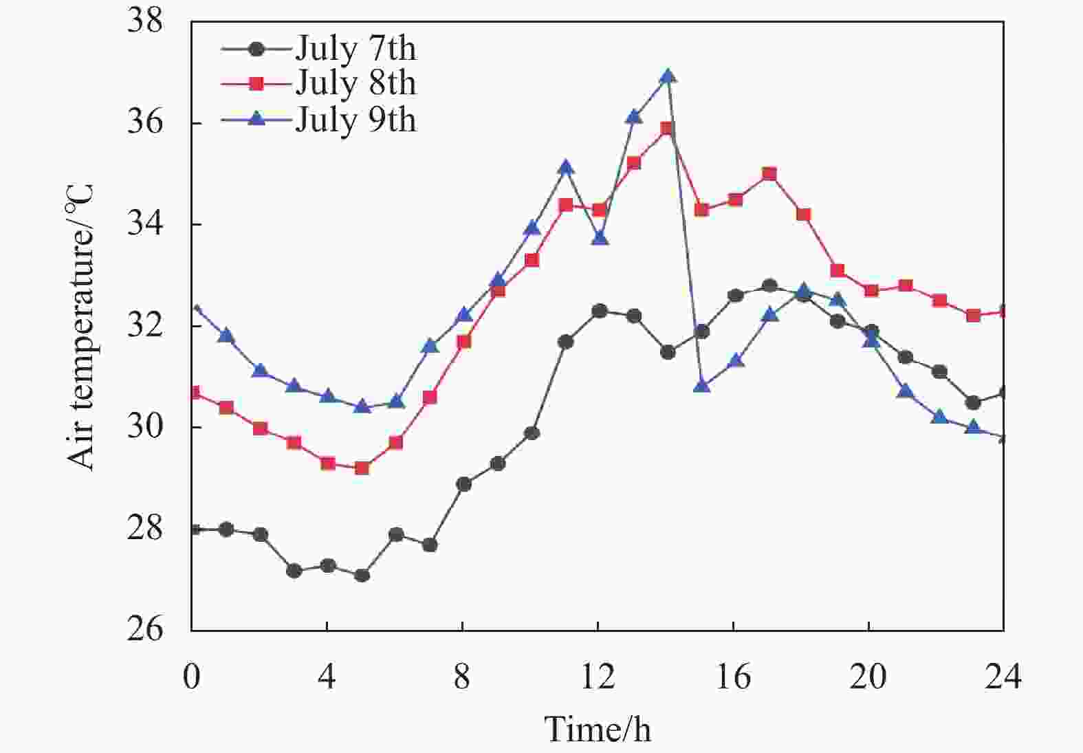
图 5 7月7日~9日空气温度变化曲线图
Figure 5. Air temperature variation curve from July 7th to 9th
-
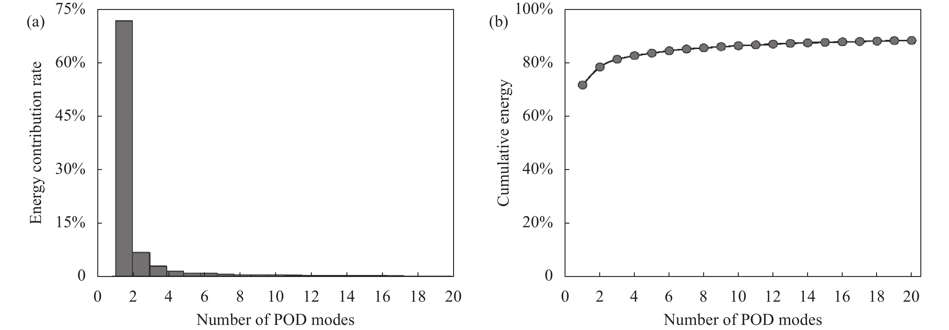
将上节处理好的温度场数据导入,将前12天的温度数据,共288组进行特征提取,通过POD,得到温度场的各阶模态,根据公式(4)、(5)计算出前20阶模态的能量贡献率和相应的模态累计率,如图6所示。
如图6(a)所示,正方腔体能量衰减得非常快,第一阶POD模态所包含的能量占比就高达71.93%,第2、3阶模态能量贡献率迅速衰减到6.75%和2.87%,前4阶模态包含了温度场的大部分特征信息,能量贡献率达到82%。随着模态数的增加,能量的衰减速率逐渐减小,最终逐渐趋于稳定。相应地,如图6(b)所示,随着POD模态数量的增加,模态的累计能量速率逐渐减小,而前16阶模态的能量贡献所占比例达到了总能量的88%,已经可以比较准确地预测出温度场,因此在进行温度场预测时应尽可能选择前16阶及以上的模态进行预测。

图 6 (a) 正方腔体前20阶POD模态能量贡献率;(b) 正方腔体前20阶模态能量累计贡献率
Figure 6. (a) Energy contribution rate of the first 20 POD modes of square cavity;(b) Cumulative energy contribution rate of the first 20 POD modes of square cavity
-
为了进一步研究POD方法对正方形腔体温度场的特征提取效果,基于上节对POD模态能量贡献率的分析,此处选择前16阶模态(蕴含温度场88%的能量)和前30阶模态(蕴含温度场90%的能量),根据公式(6)建立正方腔体温度场的降阶模型,对温度场进行预测。
图7(a)~(c)列为正方腔体真实温度场和16、30阶模态数预测的温度场。由于红外热像仪本身存在的测量误差,此处真实温度场为采集数据修正测量误差后的温度场数据,下文中计算预测误差时涉及的真实温度数据处理方法与此相同。图(a)列为2022年7月7日12时、7月8日12时、7月9日12时的真实温度场,对比图(a)列和图(b)列可以看出:前16阶模态已经能够较好地提取出正方腔体的温度场特征,并在预测其表面温度时分布趋势与真实的表面温度分布趋势基本吻合,预测的效果较好。结合图(b)、(c)列与图(a)列进行对比,在增加了POD模态后,在整体的温度图预测方面,利用前30阶模态预测出的温度图较前16阶呈现得更完善,在一些正方腔体表面呈现的热源分布上,前30阶模态在细节方面预测的效果更好。

图 7 (a)各时刻正方腔体温度场原图;(b) 16阶POD模态预测的正方腔体温度场;(c) 30阶POD模态预测的正方腔体温度场
Figure 7. (a) Original temperature field of square cavity at all times;(b) Temperature field of square cavity predicted by 16 POD modes;(c) Temperature field of square cavity predicted by 30 POD modes
由公式(8)计算出两种不同模态数的温度场预测误差,误差计算结果如表1所示。由表中数据可知,两种模态数预测出的整体误差均较小,温度场平均绝对误差均不超过1.1 K,可以实现温度场的准确预测。在相同时刻下,模态数较多相比于模态数较少预测时的误差更小。但在实际应用中,考虑到数据矩阵计算维度大等问题,前16阶模态就可满足基本的精度要求。
表 1 不同POD模态数温度场预测误差
Table 1. Temperature field prediction error with different POD modes
Time Error of 16 POD
modes/KError of 30 POD
modes/K12 o 'clock on July 7th 1.053 1.047 12 o 'clock on July 8th 1.063 1.051 12 o 'clock on July 8th 1.059 1.05 -
将POD结合QR算法应用于上述训练数据集,结合实际应用中的有限数据,通过QR算法得到最佳传感器的测量位置,通过最佳传感器的测量数据,对正方腔体的温度场进行预测,预测效果依旧用公式(8)来衡量,得到的预测误差与最佳传感器测量数量的关系如图8所示。

图 8 不同传感器个数的温度场预测误差对比
Figure 8. Comparison of temperature field prediction errors with different sensors
图8中,s为最佳传感器的测量数量,r表示POD的模态数。可以看出,温度图的预测误差随着POD模态数的增加而降低。且在相同模态数的情况下,加入QR算法得到的最佳传感器的测量数据进行预测得到的误差也较小,表明用少数传感器数据就可进行温度场的精确预测,这将大大减少计算量。
图8表明,运用少量传感器数据就可进行温度场的预测,下面将选取16个传感器、30个传感器数据对正方腔体的7月7日12时、7月8日12时的温度场进行预测,预测结果如图9和10所示。

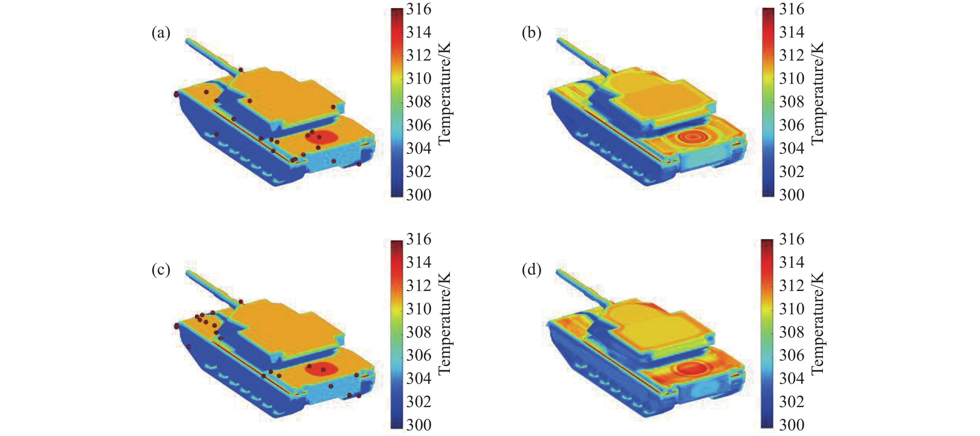
图 9 (a) 7月7日12时正方腔体传感器的分布图;(b) POD模态预测的正方腔体温度场;(c)传感器预测的正方腔体温度场
Figure 9. (a) Square cavity sensor distribution at 12:00 on July 7th; (b) Temperature field of square cavity predicted by POD mode; (c) Temperature field of square cavity predicted by sensors
如图9、10所示,图(a)~(c)列分别为温度场原图、POD预测结果、POD结合QR算法的预测结果。综合图8和图9可以看出:无论是POD预测还是POD结合QR算法,通过QR算法得到最佳传感器的测量数据进行预测,各表面的温度趋势除个别一些热源部分略有不同,其余的温度趋势以及分布的结构特点基本一致,表明两种方法都能达到很好的预测效果。若考虑到计算量的多少,则POD结合QR算法,通过QR算法得到的最佳传感器测量数据进行预测,将大大减小计算量。
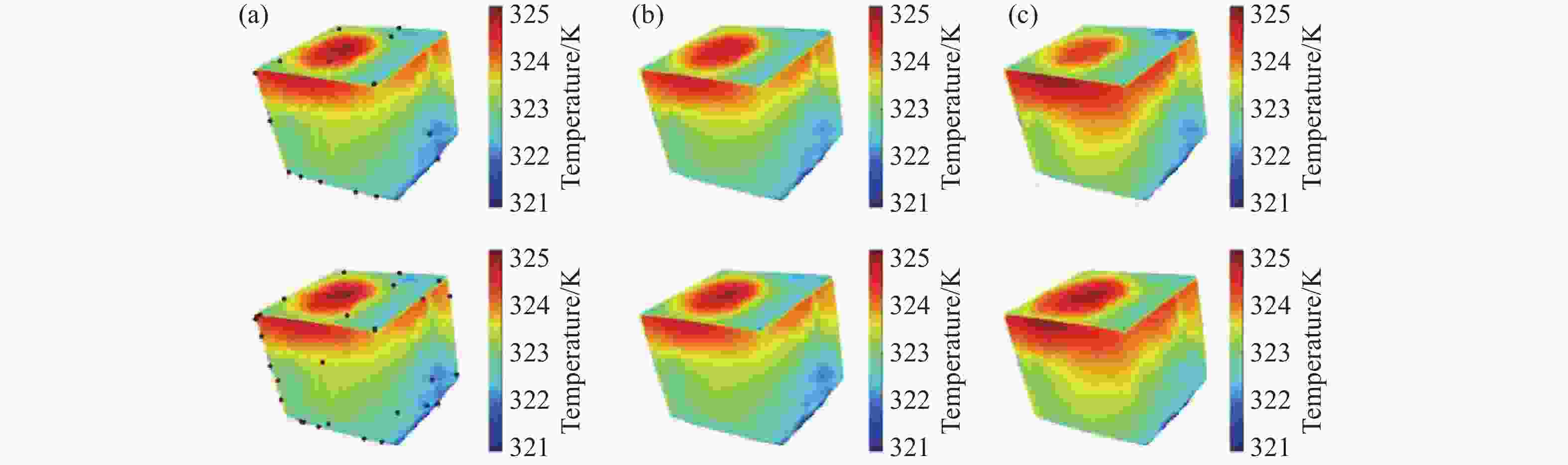
图 10 (a) 7月8日12时正方腔体传感器的分布图;(b) POD模态预测的正方腔体温度场;(c)传感器预测的正方腔体温度场
Figure 10. (a) Square cavity sensor distribution at 12:00 on July 8th; (b) Temperature field of square cavity predicted by POD mode; (c) Temperature field of square cavity predicted by sensors
为进一步分析POD以及POD结合QR算法的预测效果,在正方腔体表面选取了3个典型部位,如图11(a)所示,对其在7月7日0时~7月9日23时的真实温度值,利用前16阶POD模态和16阶POD模态结合QR算法预测出的温度值进行对比分析,3个典型部位的温度变化曲线如图11(b)~(d)所示。

图 11 (a)正方腔体表面典型部位位置示意图;(b)典型部位1;(c)典型部位2;(d)典型部位3
Figure 11. (a) Schematic diagram of typical positions on the surface of square cavity;(b) Typical position 1;(c) Typical position 2;(d) Typical position 3
由图11(b)~(d)中3条曲线的契合程度可以看出,典型部位的真实温度变化曲线趋势与16阶POD模态以及其结合QR算法预测温度的变化曲线高度契合,说明这两种方法可以很好地预测出正方腔体表面典型部位的温度,从而可以对正方腔体表面的温度分布进行很好的预测。
根据公式(8)计算出两种不同模态数及其与QR分解算法结合预测的温度场误差,得到的误差结果如表2所示。由表2可以看出,在结合QR算法得到的传感器测量数据进行预测时,无论是16个传感器和30个传感器,两种情况预测出的平均绝对误差均不超过1.5 K,误差很小且计算时间很短。可以认为,QR算法计算出的传感器测量数据能较好地代表正方腔体温度场的分布特征。30个传感器数据预测的效果较16个传感器的误差更小,传感器数据加入越多,包含的数据特征越全面,预测的效果越好。
表 2 不同传感器数量温度场的预测误差
Table 2. Temperature field prediction error with different sensors
Time Error of 16 POD modes/K Error of 16 sensors/K Error of 30 POD modes/K Error of 30 sensors/K 12 o 'clock on July 7th
1.053
1.102
1.047
1.0912 o 'clock on July 8th
1.062
1.318
1.051
1.09 -
基于上节对文中方法预测地面目标温度场的研究,考虑到实际情况下,地面目标内部热源的运行情况相对复杂,温度场数据不易获取且数据集数量较少,为了进一步研究POD方法应用于较为复杂的地面目标温度场的预测效果,设计了某型号模型坦克目标仿真试验,计算其在自然环境条件下内含内热源的温度分布,通过对不同数量温度场训练集进行POD分解,提取温度场的主要特征,从而建立温度场的降阶模型,并对不同时刻模型坦克的温度场进行预测,研究不同数量训练集对温度场的预测效果的影响。
图12(a)为模型坦克的几何模型示意图,图中所指即内热源位置,其中,内部热源为实心正方体热源,温度为1000 K,设置其在8~10时期间工作。图12(b)为带热源坦克的网格划分示意图。选取了2022年4月8日~11日的气象条件参与计算,其中的气象条件由气象观测站和太阳辐射观测站采集,采集频率为60 s/次,测试天气为多云,图13为4月8日~10日空气温度变化曲线。结合上述气象条件,利用ANSYS Fluent软件对模型坦克目标的温度场进行仿真计算。

图 12 (a) 带内热源的模型坦克目标的几何模型示意图;(b) 带内热源的模型坦克目标的网格划分示意图
Figure 12. (a) Diagram of the tank geometry model with heat producer; (b) Schematic diagram of the tank grid with heat producer

图 13 4月8日~10日空气温度变化曲线图
Figure 13. Air temperature variation curve from April 8th to 10th
-
根据仿真计算得到该模型坦克的温度场数据,由于仿真本身存在误差,由文献[16]中研究可得此类地面目标的仿真温度与真实温度误差约为1.6 K,下文中计算预测误差时将通过此误差对仿真数据进行校正,时间段为2022年4月8日1时~4月11日0时,时间间隔为1 h,温度场数量共计72组。将前24组和48组的温度数据进行特征提取,通过POD得到温度场的各阶模态,根据公式(4)、(5)计算出这两组不同数量训练集建立的温度场降阶模型的前20阶模态的能量贡献率和相应的模态累计率,如图14所示。
如图14(a)、(c)所示,与正方腔体类似,能量衰减非常快,第一阶POD模态就包含了大部分的能量,分别达到了73.17%和64.84%;24组训练集的模态能量衰减速率较48组的快;之后随着模态数的增加,能量的衰减速率逐渐减小,最终逐渐趋于一个较小的值。相应地,如图14(b)、(d)所示,随着POD模态数量的增加,图中曲线逐渐平缓,模态的累计能量增加速率逐渐减小,而对于24组训练集来说,此时前20阶模态的能量累计贡献所占比例达到了总能量的99.48%,48组训练集的前20阶模态的能量累计贡献所占比例达到了93.89%,综合两组训练集,取20阶模态已可以认为包含了温度场绝大部分的特征,可以比较准确地预测出温度场。

图 14 (a) 模型坦克24组训练集前20阶POD模态能量贡献率;(b) 模型坦克24组训练集前20阶POD模态能量累计贡献率;(c) 模型坦克48组训练集前20阶POD模态能量贡献率;(d) 模型坦克48组训练集前20阶模态能量累计贡献率
Figure 14. (a) Energy contribution rate of the first 20 POD modes of 24 trains of tank model;(b) Cumulative energy contribution rate of the first 20 POD modes of 24 trains of tank model;(c) Energy contribution rate of the first 20 POD modes of 48 trains of tank model;(d) Cumulative energy contribution rate of the first 20 POD modes of 48 trains of tank model
-
为了进一步观察不同数量训练集对POD方法预测该模型坦克温度场效果的影响,基于上节对两组不同数量训练集的POD模态能量贡献率的分析,此处对于两组不同数量训练集均选择前20阶模态(蕴含温度场90%以上的能量),根据公式(6)建立两组不同数量训练集的模型坦克温度场的POD降阶模型用于对温度场的预测。
如图15所示,图(a)列为4月10日10时、13时、20时模型坦克的温度场原图,图(b)、(c)列为24、48组训练集建立的POD降阶模型预测出的模型坦克温度场。由图15的(a)、(b)列可以看出,在温度区间相同时,根据24组训练集提取的温度场特征建立的POD降阶模型预测出的温度场与该模型坦克真实温度场分布趋势,除炮台部分以及后装甲因热源原因在表面形成的温度分布略有不同外,其余部分几乎相同,预测温度场的效果较好。结合图(b)、(c)列与图(a)列进行对比,48组训练集建立的降阶模型在炮台表面和后装甲表面热源凸显的温度分布部分预测效果更好,表明训练集数量较多的一组提取特征建立的POD降阶模型预测效果较好。
为了显著地看出两组不同数量训练集建立的POD降阶模型预测出的温度场的精确程度,根据公式(8)计算出两组降阶模型预测的温度场较原始温度场之间的误差如表3所示。
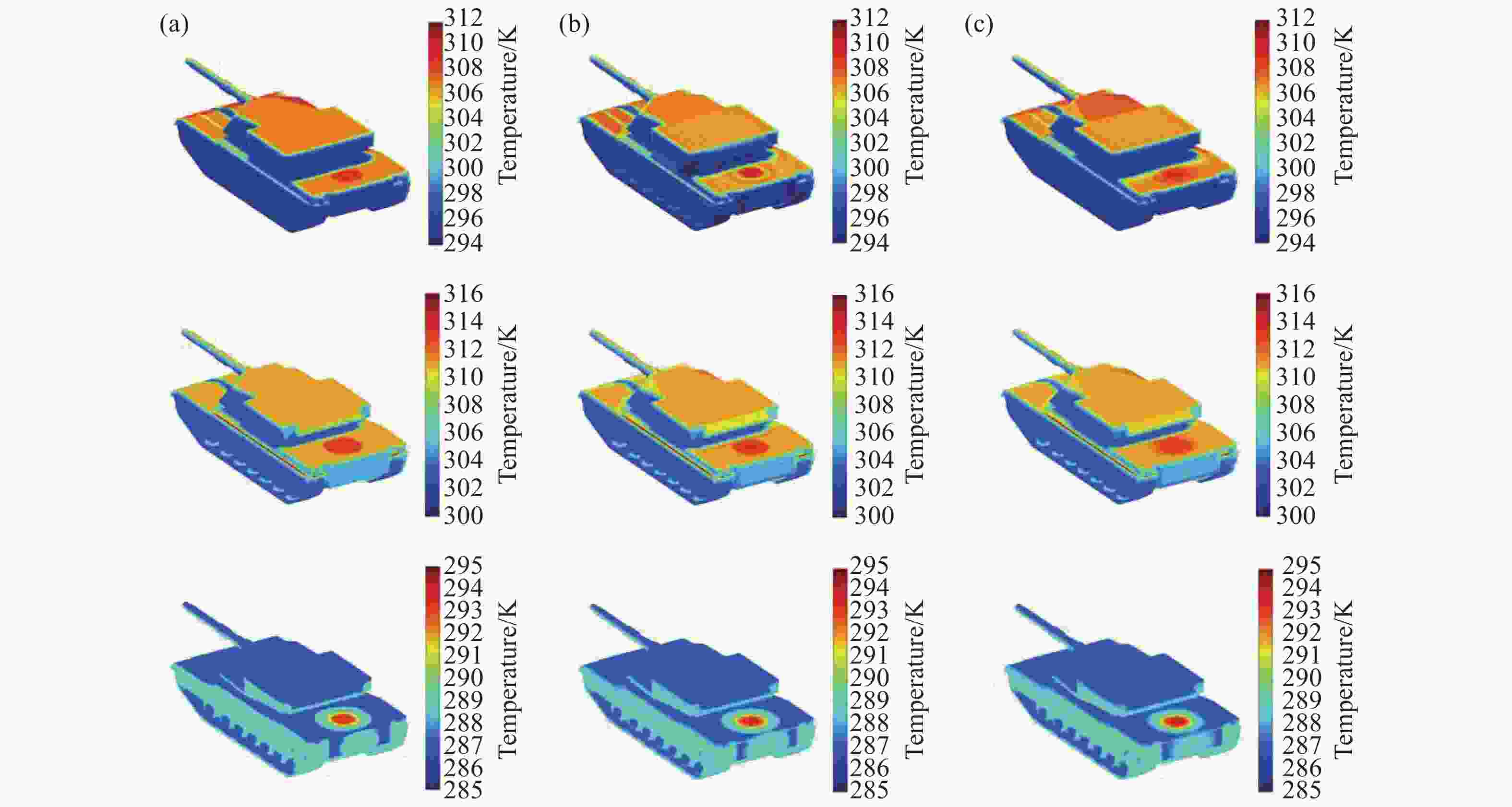
图 15 (a) 各时刻模型坦克真实温度场;(b) 模型坦克24组训练集前20阶POD模态预测的温度场;(c) 模型坦克48组训练集前20阶POD模态预测的温度场
Figure 15. (a) Original temperature field of tank at all times;(b) Temperature field of 24 trains of tank predicted by 20 POD modes;(c) Temperature field of 48 trains of tank predicted by 20 POD modes
表 3 两组降阶模型20阶POD模态温度场预测误差
Table 3. Temperature field prediction error with 20 POD modes of two reduced order models
Time Error of 24 trains/K Error of 48 trains/K 10 o 'clock on April 10th 2.2984 1.9195 13 o 'clock on April 10th 1.8625 1.8451 20 o 'clock on April 10th 1.7961 1.8004 由表3中数据可知,两组降阶模型的温度场预测的平均绝对误差均低于2.5 K,预测的准确性较高。在进行温度场预测时,训练集数量较多的一方预测的精度较训练集较少的高,由于训练集数量较多时提取的温度场特征较完善,建立的温度场降阶模型包含的温度场特征信息更多,预测的温度场更准确。在面对战场环境较为复杂的情况下,得到的地面目标温度场数据较少的情况下,利用该方法可在训练集较少时也可实现地面目标温度场较为准确的预测。
-
根据上节中两组不同数量训练集建立的降阶模型已能准确预测温度场,此处进一步研究两组降阶模型在与QR分解算法结合后对传感器分布的影响,选取30个传感器测量数据对该模型坦克4月10日13时、20时的温度场进行预测,预测结果如图16和17所示。
由图16和17可以看出,两组降阶模型与QR分解算法结合后,QR算法得到的最佳传感器的排布发生改变,与此同时利用这些传感器数据预测出的结果,相比来说,48组训练集的降阶模型得到的传感器的位置更加优化,预测出的温度场较24组训练集呈现的效果更好,更准确;从温度分布上,训练集较多的那组传感器预测结果除个别炮台部分和因热源温度凸显在后装甲表面的温度分布略有不同,其余部分基本相同,表明训练集较多时建立的降阶模型与QR分解算法计算出的最佳传感器位置更准确,预测的温度场更完善。
为了进一步观察模型坦克表面的温度变化,在模型坦克表面选取了2个典型部位,如图18(a)所示。对其在4月10日1时~4月11日0时的真实温度值、24组训练集下的POD模态以及其与QR分解算法预测出的温度值进行对比,2个典型部位的温度变化曲线如图18(b)、(c)所示。
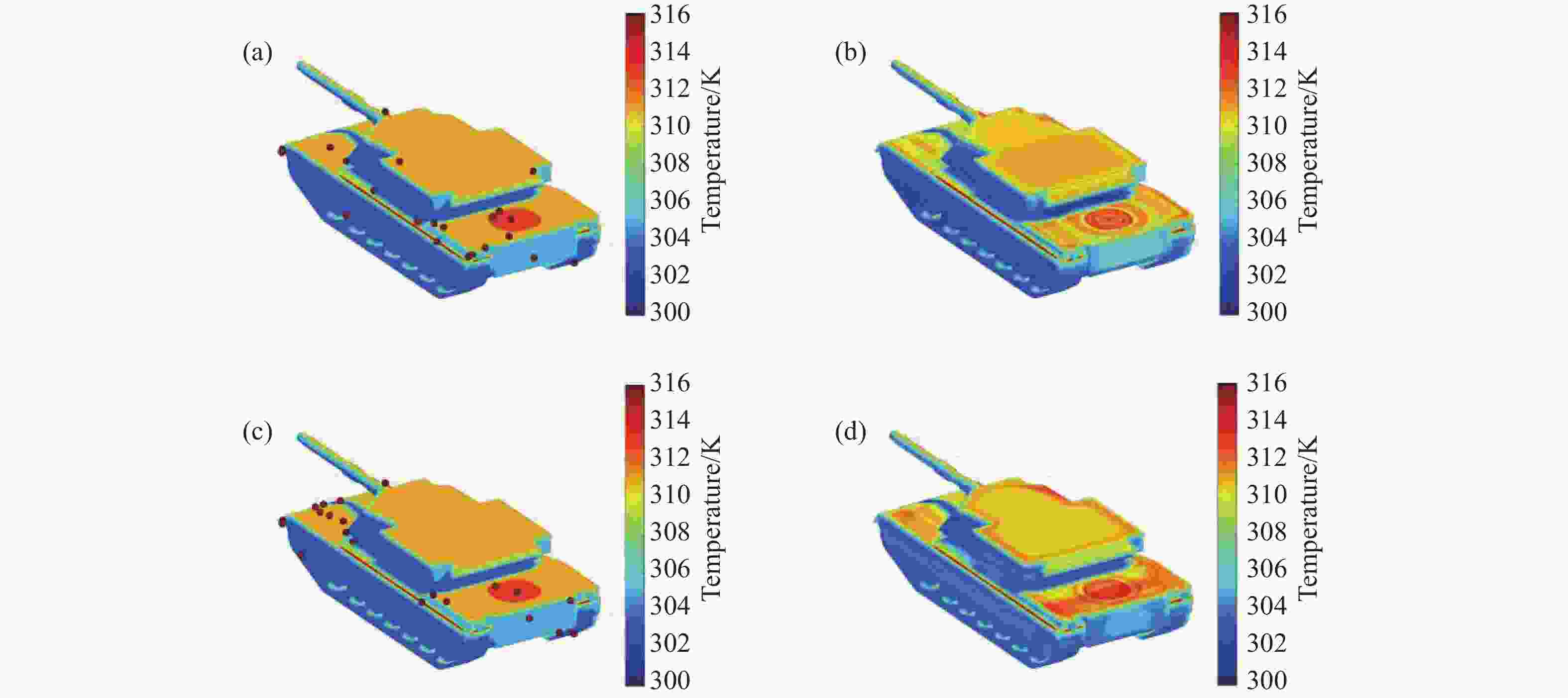
图 16 (a) 4月10日13时模型坦克24组训练集传感器的温度场分布图;(b) 模型坦克24组训练集传感器的温度场预测结果;(c) 4月10日13时模型坦克48组训练集传感器的温度场分布图;(d) 模型坦克48组训练集传感器的预测结果
Figure 16. (a) Sensor temperature field distribution of 24 trains of tank at 13:00 on April 10th;(b) Temperature field predicted result by 24 trains of tank;(c) Sensor temperature field distribution of 48 trains of tank at 13:00 on April 10th;(d) Temperature field predicted result by 48 trains of tank

图 17 (a) 4月10日20时模型坦克24组训练集传感器的温度场分布图;(b) 模型坦克24组训练集传感器的预测结果;(c) 4月10日20时模型坦克温度场48组训练集传感器的温度场分布图;(d) 模型坦克48组训练集传感器的预测结果
Figure 17. (a) Sensor temperature field distribution of 24 trains of tank at 20:00 on April 10th;(b) Temperature field predicted result by 24 trains of tank;(c) Sensor temperature field distribution of 48 trains of tank at 20:00 on April 10th;(d) Temperature field predicted result by 48 trains of tank
从图18(b)、(c)中典型部位的温度曲线走势可以看出,典型部位处的真实温度、24组训练集下的POD模态以及其与QR分解算法结合预测出的温度,这3个曲线的温度变化趋势除个别时刻预测的温度有所偏差,其余部分高度吻合,由此说明通过POD模态与POD模态结合QR分解算法得到的传感器两者预测出的典型部位处的温度均较准确。

图 18 (a)模型坦克表面典型部位位置示意图;(b)典型部位1;(c)典型部位2;
Figure 18. (a) Schematic diagram of typical positions on the surface of tank;(b) Typical position 1;(c) Typical position 2
由公式(8)计算出两组降阶模型与QR分解算法计算得到的30个传感器预测的温度场的误差,如表4所示。
表 4 两组降阶模型结合30个传感器温度场预测误差
Table 4. Temperature field prediction error with 30 sensors of two reduced order models
Time Error of 24 trains/K Error of 48 trains/K 13 o 'clock on April 10th 2.1634 2.1981 20 o 'clock on April 10th 2.13 1.9872 由表4可以看出,两组降阶模型通过与QR分解算法得到的最佳传感器测量数据预测出的温度场的平均绝对误差均低于2.5 K且计算时间较短。两个时刻,48组训练集的降阶模型与QR算法得到的传感器测量数据预测的误差均比24组训练集低,由此说明在实际情况中,利用较少的传感器数据进行温度场预测时,训练集数量较多时提取的温度场特征更完善,建立的温度场降阶模型更准确,通过QR算法得到的传感器位置更准确,从而能够更好地代表整个地面目标温度场的分布特征,预测的温度场更准确。
此外,为了定量对比出该算法的快速性,以简化模型坦克为例,分别计算并统计了不同方法下从某一时刻模型坦克温度场预测下一时刻温度场的运行时间,理论建模、POD降阶模型算法和POD降阶模型结合QR算法的运行时间如表5所示。
表 5 不同算法的运行时间
Table 5. Running time of different algorithms
Algorithms Running time/s Theoretical modeling 600 POD 8.5316 POD combined with QR 5.3495 由表5中数据可知,通过POD降阶模型和POD降阶模型结合QR算法进行预测,运行时间相较于理论建模提高了几十倍,而且通过POD降阶模型与QR算法得到的传感器测量数据进行预测的运行时间最短,说明该方法能够减少运算时间,实现利用有限测点数据实现地面目标瞬态温度场的快速预测,提高计算效率。
-
文中基于POD算法的基本理论,并将其与QR算法结合,通过QR分解算法得到最佳传感器测量数据应用于地面目标的温度场预测,以模型坦克与正方腔体两种地面目标的温度场为研究对象,对两者的温度场进行预测。得到如下结论:
1) POD方法能够很好地提取地面目标温度场的主要特征,结合模态分解时各模态的能量贡献率,可以在此基础上建立降阶模型,对地面目标温度场进行精确预测。
2)将POD与QR算法结合后,通过QR分解算法得到的最佳传感器测量数据对温度场进行预测,能够实现利用有限测点数据对地面目标温度场精确的预测,在POD温度场降阶模型的基础上,进一步减少计算时间,提高运算效率。
3)利用POD方法及其与QR分解算法结合后对两种地面目标的温度场进行预测,两种地面目标的预测温度分布与真实温度分布趋势基本相同。带热源的正方腔体温度场在16阶和30阶模态下的平均绝对误差不超过1.5 K;模型坦克目标温度场在20阶模态下的平均绝对误差不超过2.5 K,表明该方法的准确性。除此之外,在模型坦克预测中训练集较多的一组预测效果更好,位置计算更准确,计算时间也更短。
由此可见,POD可以较好地提取地面目标温度场特征,以此建立地面目标温度场的降阶模型,与QR算法结合后,通过计算出的最佳传感器测量数据实现温度场的快速精确预测,大大减少计算时间。在条件允许下可增加训练集数量和传感器个数提高准确度,为利用有限测点数据实现地面目标瞬态温度场的快速预测提供新的方法与思路。文中研究的地面目标温度场数据集时间跨度较小,且天气条件晴朗,预测的温度场时刻较为接近,未来可增加数据集的数量,以及在较为复杂的天气条件下,利用该方法建立温度场的降阶模型,开展对地面目标温度场的长期预测。将其与QR算法结合,通过QR算法得到的最佳传感器测量数据,实现利用有限测点数据对地面目标瞬态温度场的快速预测,未来可利用该方法预测目标的红外特性,为目标在战场的规避或伪装措施提供支撑。
A fast method for predicting transient temperature field of ground target based on limited measuring point data
-
摘要: 传统的地面目标红外辐射特性研究方法有理论建模分析法和外场测试法。由于大部分的理论建模计算量庞大,无法满足实时计算;外场测试往往成本较高,无法获得任意时刻地面目标整体的红外辐射特性。典型部位温度可以实时获得,但如何布置传感器使其更好地反映和预测整体的温度分布需要开展研究。文中引入本征正交分解(proper orthogonal decomposition,POD)方法对两种地面目标的温度场进行模态分析,建立两种地面目标的温度场降阶模型,利用降阶模型实现地面目标温度场的快速预测;将温度场的降阶模型与QR (orthogonal right triangular)分解算法结合,确定最佳传感器测量位置,实现对两种地面目标温度场的预测。研究结果表明,无论是POD温度场降阶模型还是通过QR分解算法得到的最佳传感器测量数据进行预测,二者的精度均较高,正方腔体的平均绝对误差均小于1.5 K,模型坦克的平均绝对误差均小于2.5 K。通过分解算法得到的最佳传感器测量数据进行预测效率更高,未来可利用该方法预测目标红外特性,从而支撑目标规避或伪装方案的制定。Abstract:
Objective With the development of infrared guidance technology, the ground targets with obvious infrared characteristics are increasingly threatened on the battlefield. In order to improve the survivability of ground targets on the battlefield, it is necessary to master the infrared radiation characteristics of ground targets. The traditional methods for studying the infrared radiation characteristics of ground targets include theoretical modeling analysis method and field testing method. The theoretical modeling analysis method is faced with such problems as a huge amount of calculation, high cost of field testing, obtained limited data, and being unable to obtain the overall infrared radiation characteristics of ground targets at any time. For the ground target, if the thermocouple is arranged on the typical part of the surface of the ground target and the relationship between the typical part and the overall temperature distribution is established, the rapid prediction of the temperature field of the ground target can be achieved. Therefore, how to arrange thermocouple on the surface of ground target and establish the relationship between the data of finite measuring points and the whole temperature field of ground target has become an urgent problem to be solved. Therefore, proper orthogonal decomposition (POD) method is introduced to extract the characteristics of the ground target temperature field, and a reduced order model of the temperature field is established. On this basis, combined with QR (orthogonal right triangular) decomposition algorithm, the rapid prediction of the temperature field of the ground target is realized by using the data of finite measuring points. Methods POD method is introduced into temperature field characteristics analysis of ground targets, and the specific implementation process is shown (Fig.1). Taking square cavity and model tank as the research objects, POD method was used to extract the temperature field characteristics of ground targets, and two kinds of ground target temperature field reduction models were established to predict the temperature distribution of ground targets at multiple moments and compare it with the real temperature field at the same moment (Fig.7, Fig.15). Based on the reduced order model of temperature field combined with QR decomposition algorithm, the position of the best sensor was determined, and the temperature field was predicted by using the measured data of the best sensor, and compared with the real temperature field (Fig.9-10, Fig.16-17). Finally, the reliability of the method is verified by error calculation and analysis. Results and Discussions POD method can extract the main characteristics of the ground target temperature field well. On this basis, the reduced order model is established, and the predicted temperature distribution is basically consistent with the real ground target temperature distribution. After combining POD and QR algorithm, the best sensor measurement data obtained by QR decomposition algorithm is used to predict the temperature field of two ground targets. The predicted temperature distribution trend of the two ground targets is basically the same as the real temperature distribution trend. Based on the POD temperature field reduction model, the calculation time is further reduced and the calculation efficiency is improved. The average absolute error of the temperature field of the square cavity with heat source is less than 1.5 K. The average absolute error of the temperature field of the model tank target is less than 2.5 K. This indicates the accuracy of the method. Conclusions It can be seen that POD can better extract the characteristics of the temperature field of the ground target, so as to establish the reduced order model of the temperature field of the ground target. After combining with the QR algorithm, the temperature field can be quickly and accurately predicted through the calculated best sensor measurement data, greatly reducing the calculation time. If conditions permit, the number of training sets and sensors can be increased to improve the accuracy, which provides a new method and idea for the rapid prediction of transient temperature field of ground targets by using finite measuring point data. -
图 2 数据处理流程示意图(正方腔体温度场)
Figure 2. Data processing flow diagram (square cavity temperature field)
图 4 (a) 正方腔体含背景温度图;(b) 正方腔体去除背景温度图
Figure 4. (a) Diagram of square cavity with background temperature;(b) Diagram of square cavity removed background temperature
图 6 (a) 正方腔体前20阶POD模态能量贡献率;(b) 正方腔体前20阶模态能量累计贡献率
Figure 6. (a) Energy contribution rate of the first 20 POD modes of square cavity;(b) Cumulative energy contribution rate of the first 20 POD modes of square cavity
图 7 (a)各时刻正方腔体温度场原图;(b) 16阶POD模态预测的正方腔体温度场;(c) 30阶POD模态预测的正方腔体温度场
Figure 7. (a) Original temperature field of square cavity at all times;(b) Temperature field of square cavity predicted by 16 POD modes;(c) Temperature field of square cavity predicted by 30 POD modes
图 8 不同传感器个数的温度场预测误差对比
Figure 8. Comparison of temperature field prediction errors with different sensors
图 9 (a) 7月7日12时正方腔体传感器的分布图;(b) POD模态预测的正方腔体温度场;(c)传感器预测的正方腔体温度场
Figure 9. (a) Square cavity sensor distribution at 12:00 on July 7th; (b) Temperature field of square cavity predicted by POD mode; (c) Temperature field of square cavity predicted by sensors
图 10 (a) 7月8日12时正方腔体传感器的分布图;(b) POD模态预测的正方腔体温度场;(c)传感器预测的正方腔体温度场
Figure 10. (a) Square cavity sensor distribution at 12:00 on July 8th; (b) Temperature field of square cavity predicted by POD mode; (c) Temperature field of square cavity predicted by sensors
图 11 (a)正方腔体表面典型部位位置示意图;(b)典型部位1;(c)典型部位2;(d)典型部位3
Figure 11. (a) Schematic diagram of typical positions on the surface of square cavity;(b) Typical position 1;(c) Typical position 2;(d) Typical position 3
图 12 (a) 带内热源的模型坦克目标的几何模型示意图;(b) 带内热源的模型坦克目标的网格划分示意图
Figure 12. (a) Diagram of the tank geometry model with heat producer; (b) Schematic diagram of the tank grid with heat producer
图 13 4月8日~10日空气温度变化曲线图
Figure 13. Air temperature variation curve from April 8th to 10th
图 14 (a) 模型坦克24组训练集前20阶POD模态能量贡献率;(b) 模型坦克24组训练集前20阶POD模态能量累计贡献率;(c) 模型坦克48组训练集前20阶POD模态能量贡献率;(d) 模型坦克48组训练集前20阶模态能量累计贡献率
Figure 14. (a) Energy contribution rate of the first 20 POD modes of 24 trains of tank model;(b) Cumulative energy contribution rate of the first 20 POD modes of 24 trains of tank model;(c) Energy contribution rate of the first 20 POD modes of 48 trains of tank model;(d) Cumulative energy contribution rate of the first 20 POD modes of 48 trains of tank model
图 15 (a) 各时刻模型坦克真实温度场;(b) 模型坦克24组训练集前20阶POD模态预测的温度场;(c) 模型坦克48组训练集前20阶POD模态预测的温度场
Figure 15. (a) Original temperature field of tank at all times;(b) Temperature field of 24 trains of tank predicted by 20 POD modes;(c) Temperature field of 48 trains of tank predicted by 20 POD modes
图 16 (a) 4月10日13时模型坦克24组训练集传感器的温度场分布图;(b) 模型坦克24组训练集传感器的温度场预测结果;(c) 4月10日13时模型坦克48组训练集传感器的温度场分布图;(d) 模型坦克48组训练集传感器的预测结果
Figure 16. (a) Sensor temperature field distribution of 24 trains of tank at 13:00 on April 10th;(b) Temperature field predicted result by 24 trains of tank;(c) Sensor temperature field distribution of 48 trains of tank at 13:00 on April 10th;(d) Temperature field predicted result by 48 trains of tank
图 17 (a) 4月10日20时模型坦克24组训练集传感器的温度场分布图;(b) 模型坦克24组训练集传感器的预测结果;(c) 4月10日20时模型坦克温度场48组训练集传感器的温度场分布图;(d) 模型坦克48组训练集传感器的预测结果
Figure 17. (a) Sensor temperature field distribution of 24 trains of tank at 20:00 on April 10th;(b) Temperature field predicted result by 24 trains of tank;(c) Sensor temperature field distribution of 48 trains of tank at 20:00 on April 10th;(d) Temperature field predicted result by 48 trains of tank
图 18 (a)模型坦克表面典型部位位置示意图;(b)典型部位1;(c)典型部位2;
Figure 18. (a) Schematic diagram of typical positions on the surface of tank;(b) Typical position 1;(c) Typical position 2
表 1 不同POD模态数温度场预测误差
Table 1. Temperature field prediction error with different POD modes
Time Error of 16 POD
modes/KError of 30 POD
modes/K12 o 'clock on July 7th 1.053 1.047 12 o 'clock on July 8th 1.063 1.051 12 o 'clock on July 8th 1.059 1.05  下载: 导出CSV
表 2 不同传感器数量温度场的预测误差
Table 2. Temperature field prediction error with different sensors
Time Error of 16 POD modes/K Error of 16 sensors/K Error of 30 POD modes/K Error of 30 sensors/K 12 o 'clock on July 7th
1.053
1.102
1.047
1.0912 o 'clock on July 8th
1.062
1.318
1.051
1.09
下载: 导出CSV
表 3 两组降阶模型20阶POD模态温度场预测误差
Table 3. Temperature field prediction error with 20 POD modes of two reduced order models
Time Error of 24 trains/K Error of 48 trains/K 10 o 'clock on April 10th 2.2984 1.9195 13 o 'clock on April 10th 1.8625 1.8451 20 o 'clock on April 10th 1.7961 1.8004
下载: 导出CSV
表 4 两组降阶模型结合30个传感器温度场预测误差
Table 4. Temperature field prediction error with 30 sensors of two reduced order models
Time Error of 24 trains/K Error of 48 trains/K 13 o 'clock on April 10th 2.1634 2.1981 20 o 'clock on April 10th 2.13 1.9872
下载: 导出CSV
表 5 不同算法的运行时间
Table 5. Running time of different algorithms
Algorithms Running time/s Theoretical modeling 600 POD 8.5316 POD combined with QR 5.3495
下载: 导出CSV
-
[1] Sui Juncheng, Ren Dengfeng, Han Yuge. Inversion and model validation method of missing parameters in infrared modeling of ground targets [J]. Infrared and Laser Engineering, 2022, 51(10): 20220033. (in Chinese) doi: 10.3788/IRLA20220033 [2] Luo Qingguo, Lu Jun, Zhao Yao. Analysis of thermal flow field and infrared radiation characteristics of tank power cabin [J]. Laser & Infrared, 2020, 50(1): 74-79. (in Chinese) doi: 10.3969/j.issn.1001-5078.2020.01.014 [3] Zhao Yao, Luo Qingguo, Lu Jun, et al. Temperature field and infrared radiation characteristics for armored vehicle engine compartment [J]. Journal of Academy of Armored Force Engineering, 2018, 32(4): 34-39. (in Chinese) [4] Li Junshan, Chen Xia, Li Jianhua. Infrared radiation charac-teristics contrast between target and background on different grounds [J]. Infrared and Laser Engineering, 2014, 43(2): 424-428. (in Chinese) [5] Lv Zhenhua, Pan Xiaoli, Gong Guanghong, et al. Research terrain background infrared radiation characteristics modeling and simulation [J]. Journal of Journal of China Academy of Electronics and Information Technology, 2017, 12(4): 420-427. (in Chinese) [6] 孙晓霞, 卫朝富. 地面目标与背景红外特性测试现场快速评估方法[J]. 兵器装备工程学报, 2020, 41(04): 196-202. doi: 10.11809/bqzbgcxb2020.04.038 Sun Xiaoxia, Wei Chaofu. Fast field evaluation method for ground target and background infrared characteristics test [J]. Journal of Ordnance Equipment Engineering, 2020, 41(4): 196-202. (in Chinese) doi: 10.11809/bqzbgcxb2020.04.038 [7] Cheng Shengyue, Liu Zhaohui, Deng Zhiping, et al. Research progress on infrared characteristic of military target [J]. Infrared Technology, 2014, 36(7): 577-581. (in Chinese) [8] Alexandros Iliopoulos, Rasoul Shirzadeh, Wout Weijtjens, et al. A modal decomposition and expansion approach for prediction of dynamic responses on a monopile offshore wind turbine using a limited number of vibration sensors [J]. Mechanical Systems and Signal Processing, 2016, 68-69: 84-104. doi: https://doi.org/10.1016/j.ymssp.2015.07.016 [9] Zhang Xiaohua, Zhou Haiyang. Multi-type structural responses reconstruction using limited number of sensors [J]. Journal of Nanchang University (Engineering & Technology), 2016, 38(2): 147-151. (in Chinese) [10] Chen M, Liu S, Sun S, et al. Rapid reconstruction of simulated and experimental temperature fields based on proper orthogonal decomposition [J]. Applied Sciences, 2020, 10(11): 3729. doi: 10.3390/app10113729 [11] Mokhasi P, Rempfer D. Optimized sensor placement for urban flow measurement [J]. Physics of Fluids, 2004, 16(5): 1758-1764. doi: 10.1063/1.1689351 [12] Manohar K, Brunton B W, Kutz J N, et al. Data-driven sparse sensor placement for reconstruction: demonstrating the benefits of exploiting known patterns [J]. IEEE Control Systems Magazine, 2018, 38(3): 63-86. doi: 10.1109/MCS.2018.2810460 [13] Manohar K, Kutz J N, Brunton S L. Optimal sensor and actuator selection using balanced model reduction [J]. IEEE Transactions on Automatic Control, 2022, 67(4): 2108-2115. doi: 10.1109/TAC.2021.3082502 [14] Manohar K, Kaiser E, Brunton S L, et al. Optimized sampling for multiscale dynamics [J]. Multiscale Modeling & Simulation, 2019, 17(1): 117-136. doi: https://doi.org/10.1137/17M1162366 [15] Nakai K, Yamada K, Nagata T, et al. Effect of objective function on data-driven greedy sparse sensor optimization [J]. IEEE Access, 2021, 9: 46731-46743. doi: 10.1109/ACCESS.2021.3067712 [16] Lin Qunqing. Research on the effects of droplets and particles on thermal radiative characteristics of vehicles and credibility evaluation method for thermal radiation model[D]. Nanjing: Nanjing University of Science and Technology, 2018. (in Chinese) -

 点击查看大图

计量
- 文章访问数: 49
- HTML全文浏览量: 10
- PDF下载量: 21
- 被引次数: 0

