近年来，拓扑光子学领域的研究引起了广泛关注，其中一个重要分支便是对外尔点的研究。作为一种无质量的相对论费米子，外尔费米子在量子理论和标准模型中发挥着重要的作用。人们发现在打破时间反演对称性或者空间反演对称性的结构中，动量空间会出现受拓扑保护的外尔点，并可以用于类比外尔费米子的物理特性^[1-2]。在三维动量空间中，两条线性色散的能带互相接触构成外尔点，这类二重简并点具有鲁棒性。外尔点具有很多独特的性质，例如，手性正负的外尔点分别对应贝利曲率的源和漏，因此，外尔点也被认为是动量空间的磁单极子^[3-4]。自然界中具有外尔点的材料通常被称为外尔半金属^[5-6]。在外尔半金属的界面上，非平庸表面态费米弧的存在是判定材料为外尔半金属的一大证据。除此之外，外尔半金属还具有手征反常^[7-8]、手征零能模式^[9-10]、螺旋表面态^[11-13]等独特的现象。

超材料是指将人工设计的亚波长结构以特定方式排列。由于可以人为设计、任意控制，能实现各种自然界难以出现的电磁特征，超材料现已被广泛应用于各个研究领域^[14-15]，并已取得丰硕的成果，例如超透镜、高性能天线等。在微波波段，利用等效介质理论，可以合理设计各向异性的介电常数$\varepsilon $、磁导率$ \mathrm{\mu } $等参数，在能带结构中引入简并点、简并线、椭圆色散、双曲色散等^[16-18]特殊性质。基于空间反演对称性破缺这一要求，可以在微波波段设计出能带结构具有外尔点的超材料，为后续研究提供平台。

基于人工设计构建出的外尔超材料，笔者将讨论外尔超材料与空气界面的反射本征态。后续部分将按照如下顺序进行叙述：首先，对外尔超材料的电磁本构关系进行求解，接着论述反射本征态的定义与计算方法，最后展示外尔超材料与空气界面的反射本征态的求解结果。令人惊奇的是，在入射电磁场为线性偏振模式的前提下，外尔超材料的反射本征场在整个布里渊区范围内均为线性偏振模式，这一现象是由系统能量守恒与洛伦兹互易性共同保证的。

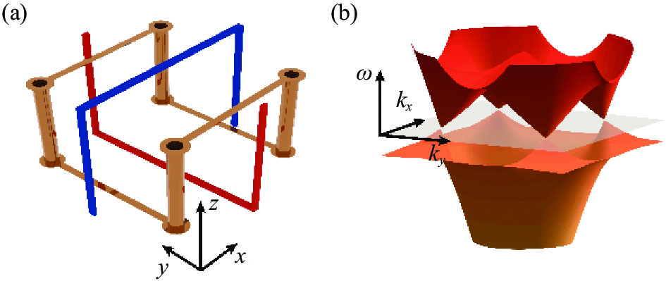
笔者利用理想外尔超材料^{[9, 12, 18]}进行后续的研究。这种外尔超材料具有十分优越的能带结构：在同一频率有4个第一类外尔点，并且在外尔点频率附近，没有其他的非拓扑能带干扰，这样的能带结构为探究外尔点的基础性质提供了很好的平台。

外尔超材料由结构单元平移构成，结构单元主体为马鞍型金属结构，如图1（a）金色部分所示。马鞍型金属结构具有$ {D}_{2 d} $点群对称，这样的结构打破了空间反演对称性。金属结构外部包裹有各向同性背景材料。由于背景材料仅起支撑作用，在此没有画出。通过将结构单元周期性排列，应用仿真软件，可以计算得到外尔超材料的本征频率随动量的变化，即外尔超材料的能带结构。图1（b）是外尔点频率附近的能带结构图，灰色半透明面标注外尔点频率的等频面，能带结构与等频面的交点只有4个外尔点，意味着在该频率除了外尔点以外，没有其他本征态。

图  1  （a） 马鞍型金属结构与等效开口环共振模型；（b）理想外尔超材料的能带结构：4个外尔点在同一频率

Figure 1.  (a) Saddle shaped metallic structure and effective split ring resonator model; (b) Band structure of ideal Weyl metamaterial: four Weyl nodes located at the same frequency

利用等效介质理论，马鞍型金属结构的电磁场特性可以十分简洁的形式来描述。马鞍型金属结构单元可以被等效为两个开口环共振结构（SRR）互相嵌套在一起，见图1（a）。其中蓝色开口环与红色开口环互相垂直、朝向相反，其余几何参数则完全相同。依据文献[12]中的等效介质理论，考虑金属开口环在外电磁场中的电子响应，写出连续参数变化的理论描述。为了简化运算，设置$ {\varepsilon}_{0}={\mu }_{0}=c=1 $。由此，利用RLC电路模型，两个开口环的电流I和电荷分布q可以被写成如下形式：

式中：$ {a} $为开口环的面积；${l} $为边长；开口环的本征共振频率为$ {\omega }_{0}=\dfrac{1}{\sqrt{LC}} $，L和C分别为电感和电容；$ \mathrm{\omega },{E},{H} $分别为外电场的频率以及电场、磁场面内场的分量。这里考虑没有损耗的情况，取电阻为零$R= 0,\gamma =\dfrac{R}{L}=0$。麦克斯韦方程组可写为：

其中，电磁耦合项写为：

由此写出马鞍型金属结构的本构矩阵为：

接下来，在外尔点频率，考虑半无限外尔超材料与空气界面的反射：${z} < 0 $为外尔超材料，${z} > 0 $为空气（均匀介质），${z}=0 $的平面为外尔超材料与空气的分界面。由于除了外尔点以外，该频率不存在其他能带，在动量空间内材料体现出全反射特性，入射态空间与反射态空间的能量守恒，透射态空间能量为零。

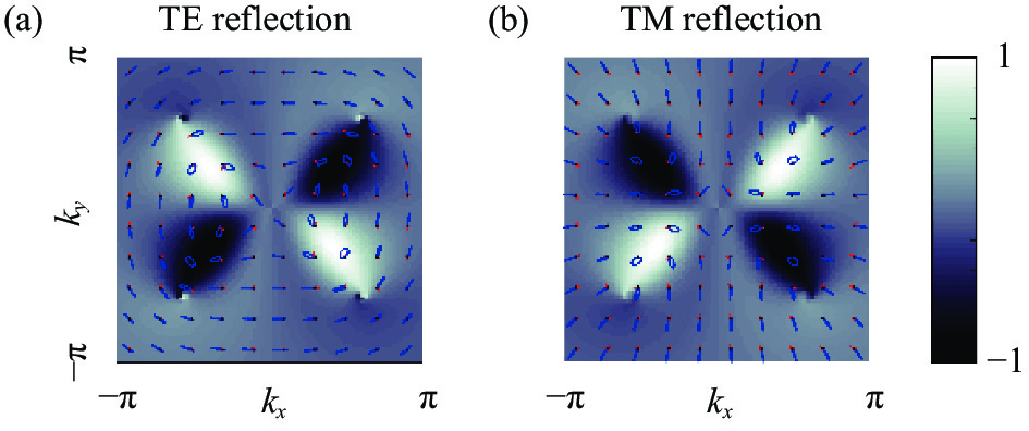
外尔超材料具有偏振转换特性，当入射电磁场为线性偏振模式时，在外尔点附近反射场出现了椭圆偏振，见图2。箭头表示偏振态电磁场分布及分量的相位关系，在靠近布里渊区边界时，反射电磁场为线偏振模式，而外尔点附近则出现了椭圆偏振模式。图2的底色表示斯托克斯参量$ {S}_{3}=2{E}_{x}{E}_{y}\sin \Delta $，用以表征偏振态椭圆度在布里渊区内的变化：x方向电场分量与y方向相位差越大，$ \left|{{S}}_{3}\right| $越大，$ {{S}}_{3}=\pm 1 $为圆偏振光；若偏振态为线性模式，则$ {{S}}_{3}=0 $。以图2（a）为例，在靠近布里渊区边界的地方，图片底色呈现灰色，$ {{S}}_{3}=0 $，说明入射电磁场为TE模式，反射得到仍是线性偏振模式；而在靠近左上角外尔点的位置，图片底色接近白色，说明当入射电磁场为线偏振模式时， $ {{S}}_{3} $接近1，反射得到的是椭圆偏振模式，入射模式与出射模式对比发生了偏振转换。值得一提的是，左上角与右下角的外尔点手性相同，反射场的性质也类似。对于整个二维布里渊区而言，反射场满足$ {{C}}_{2} $旋转对称性。

图  2  外尔超材料的反射电磁场。（a） TE模式入射；（b） TM模式入射，背景为斯托克斯参量${{S}} _{3}$分量

Figure 2.  Reflection electromagnetic field of Weyl metamaterial. (a) TE mode incident; (b) TM mode incident. The background color indicates the S₃

根据边界连续条件，在给定入射电磁场的前提下，反射电磁场是唯一确定的。但需要注意的是，入射态空间与反射态空间的波矢并不相同，在均匀介质的界面，不考虑高阶散射，若入射波矢为$\overrightarrow{{{k} }}_{{i}{n}}=[{{k}}_{{x}},{{k}}_{{y}},{{k}}_{{z}}]$，对应的反射波矢则是$\overrightarrow{{{k }}}_{{r}{e}{f}}=[{{k}}_{{x}},{{k}}_{{y}},{-{k}}_{{z}}]$，反射波矢与入射波矢相比，垂直于界面的波矢分量方向相反。所有入射电磁场均定义在入射波矢$\overrightarrow{{{k} }}_{{i}{n}}=[{{k}}_{{x}},{{k}}_{{y}},{{k}}_{{z}}]$的前提下，与反射电磁场属于不同的态空间。因此，对于入射电磁场与反射电磁场这两个不同的态空间，需要分别定义电磁场基矢，用以描述入射和反射模式。

经过界面反射后，对比反射波矢与入射波矢，只有垂直于界面的分量符号发生改变，平行于界面的分量保持不变。因此，笔者定义镜像算符$ \widehat{{M}} $将入射波矢与反射波矢联系起来，从而建立起入射态空间与反射态空间两者的联系。

在每个态空间，需要两个线性无关的电磁场模式来构成一组基矢，例如，在电磁场分析中，常用一组线性偏振态$ \left|{T}{E}\right\rangle, \left|{T}{M}\right\rangle $作为基矢。在入射态空间，用$ \left|{{{\rm{Down}}}}_{1}\right\rangle, \left|{{{\rm{Down}}}}_{2} \right\rangle $来表示任意一组基矢，入射态空间所有可能的电磁场模式均可以表示为这组基矢的线性叠加。此处$ \left|{{{\rm{Down}}}}_{1}\right\rangle, \left|{{{\rm{Down}}}}_{2}\right\rangle $不限定为线偏振模式，两个线性无关的椭圆偏振模式、或者左旋圆偏振光与右旋圆偏振光也可以构成一组基矢。

入射模式基矢$\left|{{{\rm{Down}}}}_{1}\right\rangle, \left|{{{\rm{Down}}}}_{2} \right\rangle$对应的反射模式分别记为$\left|{\mathrm{U}\mathrm{p}}_{1}\right\rangle,\left|{\mathrm{U}\mathrm{p}}_{2}\right\rangle$，

入射态空间与反射态空间是同构的，因此$ \left|{\mathrm{U}\mathrm{p}}_{1}\right\rangle, \left|{\mathrm{U}\mathrm{p}}_{2}\right\rangle $也是一组线性无关的模式，可以成为反射态空间的一组基矢。

镜像算符定义为，$\widehat{M}\left|{{\rm{Down}}}_{i}\right\rangle=\left|{{\rm{Up}}}_{{i}}\right\rangle,i=\mathrm{1,2}$。波矢与电场均是极矢量(polar vector)，见图3（a），在镜像操作下平行界面的分量保持不变，垂直界面分量的符号反向，即

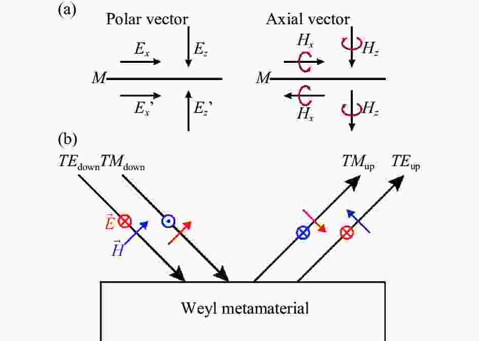
图  3  （a）极矢量与轴矢量；（b）一组本征态

Figure 3.  (a) Polar vector and axial vector; (b) Illustration of a set of basis

而磁场是由极矢量向量积定义($ \overrightarrow{{k}}\times \overrightarrow{{E}} $)，为轴矢量(axis vector)，在镜像操作下平行于界面的分量符号反向，而垂直于界面分量则保持不变，

结合电场分量与磁场分量经由界面反射后，分量符号的变化规律，写出$ \left|{\mathrm{U}\mathrm{p}}_{1}\right\rangle,\left|{\mathrm{U}\mathrm{p}}_{2}\right\rangle $的分量形式为：

由此，镜像算符$ \widehat{M} $的具体形式可以写为：

式中：$ \widehat{K} $为共轭算符。镜像算符用于在入射态空间与反射态空间之间相互转化，例如：

如图3（b）所示，不失一般性，笔者选取常见的线性偏振模式$ \left|{TE}_{{\rm{down}}}\right\rangle, \left|{TM}_{{\rm{down}}}\right\rangle $作为入射态空间的基矢，对应的反射态空间基矢为：

红色箭头表示电场分量，蓝色箭头表示磁场分量，黑色箭头则是波矢方向，入射电磁场基矢与反射电磁场基矢通过$ \widehat{{M}} $互相转化。

需要注意的是，镜像算符$ \widehat{{M}} $仅仅是联系入射态空间与反射态空间的诸多方式中的一种，在其他文献中亦有另外的定义方式。对于相同的入射电磁场而言，材料的反射电磁场是唯一确定的，不同的基矢定义方式并不会改变反射场，只是将场分量以不同基矢展开。

该节将展示在利用镜像算符$ \hat{M}̂$联系两个态空间的前提下，讨论以线偏振模式$ \left|{{T}{E}}_{\mathrm{d}\mathrm{o}\mathrm{w}\mathrm{n}}\right\rangle, \left|{{T}{M}}_{\mathrm{d}\mathrm{o}\mathrm{w}\mathrm{n}}\right\rangle $入射，外尔超材料在外尔频率的反射本征态必然是线性的。

首先，对反射本征态进行定义。用$ \widehat{{R}} $表示界面反射算符，则入射$ \left|{{T}{E}}_{\mathrm{d}\mathrm{o}\mathrm{w}\mathrm{n}}\right\rangle $得到的反射电磁场可以用$ \left|T{E}_{{\rm{up}}}\right\rangle,\left|T{M}_{{\rm{up}}}\right\rangle $进行展开，入射场为$ \left|T{M}_{{\rm{down}}}\right\rangle $同理，展开方程如下：

式中：$ {a},{b},{c},{d} $为展开系数。为了求解方程组，需要先将等式两边基矢变换到同一态空间，应用镜像算符$ \widehat{{M}} $进行基矢变换，

此时可以写出界面反射算符与镜像算符的矩阵表示为：

式中：$ i,j=1,\left|{r}_{1}\right\rangle=\left|T{E}_{{\rm{up}}}\right\rangle $,$ i,j=2,\left|{r}_{2}\right\rangle=\left|T{M}_{{\rm{up}}}\right\rangle $，此时反射系数矩阵为：

需要注意的是，反射系数矩阵是$\widehat{{R}}\widehat{{M}}$的矩阵表示，而不是$ \widehat{{R}} $的矩阵表示。

对反射系数矩阵进行对角化，可以求得两个本征态以及对应的本征值。由于系统能量守恒，反射系数矩阵为酉矩阵，两个本征值记为：

以第一个本征态为例，$D\left|{\phi }_{1}\right\rangle= \rm{e}^{i{\phi }_{1}}\left|{\phi }_{1}\right\rangle$，$ \left|{\phi }_{1}\right\rangle $为本征矢量。反射系数矩阵的本征矢量$ \left|{\phi }_{1}\right\rangle $为$ 2\times 1 $的矢量，含义为对应基矢的系数。将基矢系数与基矢相乘的结果线性叠加，便可得到反射态空间中电磁场模式的形式为：

入射态空间与反射态空间通过镜像算符$ \widehat{M} $关联，入射态空间内的电磁场形式为：

上述的界面反射过程可以记为：

此处反射系数矩阵本征态可以理解为：当入射电磁场为$\widehat{{M}}\left|EH\right\rangle$时，反射模式便是$ \left|EH\right\rangle $并具有额外相位${\rm e}^{i{\phi }_{1}}$，因此，将反射本征态写为：

反射本征态定义在反射态空间内，其入射态空间的对应本征态为：

在这样的定义下，外尔超材料的两个本征态必然是线性的，见图4。当入射基矢取$\left|{{T}{E}}_{{{\rm{down}}}}\right\rangle, \left| T{M}_{{{\rm down}}}\right\rangle$时，反射系数矩阵的独特性质会直接导出线性本征态的结果。

图  4  外尔超材料反射本征态的电磁场为线性偏振模式

Figure 4.  Reflection eigen electromagnetic fields of Weyl metamaterial are linear polarized

反射系数矩阵的一般形式为：

在系统没有损耗的前提下，反射系数矩阵为酉矩阵，以满足能量守恒的要求。因此，采用酉矩阵通用形式，可以将反射系数矩阵记为$ A=U\lambda {U}^{-1} $，其中${U}$代表矩阵${A}$的本征矢量矩阵，$ \mathrm{\lambda } $代表本征值，

根据酉矩阵的性质，有$ U\in U\left(2\right) $，$ {U}^{-1}={{U}^{\mathrm{*}}}^{{\rm{T}}} $，

由于该界面的反射过程满足洛伦兹互易，反射系数矩阵是对称矩阵，即$ {A}^{{\rm{T}}}=A $，

因此，本征矢量${U} $内元素必须均为实数。由于本征矢量${U} $的物理意义为基矢$ \left|{{T}{E}}_{{{\rm{up}}}}\right\rangle,\left|T{M}_{{\rm{up}}}\right\rangle $的系数，而基矢$ \left|{{T}{E}}_{{{\rm{up}}}}\right\rangle,\left|T{M}_{{\rm{up}}}\right\rangle $为线性偏振模式，每个分量均为实数，因此，本征态必然为线性偏振模式，图4(a)和(b)分别对应两个反射本征模式，红点为外尔点，箭头表示电磁场，所有的箭头都是线性的，没有出现椭圆偏振态与圆偏振态的情况。

在第一布里渊区里，可以看到本征态的电磁场并不是朝向一致的，如图4所示。由于外尔点（红色圆点）是反射相位奇点，本征电磁场的方向在外尔点附近剧烈变化。在右上角外尔点附近取圆形路径，环绕外尔点进行扫描，得到本征电磁场朝向变化如图5（a）所示。所有反射本征态均为线性偏振模式，线段颜色表示本征态的相位${\mathrm{e}}^{{i}\mathrm{\phi }}$。在每一点都有两个本征态，两个反射本征态所对应的本征相位不同，同时这两个本征态电磁场方向互相垂直，构成十字叉形。随着扫描路径在布里渊区位置的连续改变，十字叉形的朝向也在连续变化。值得一提的是，当扫描路径在动量空间绕外尔点一圈时，本征电磁场方向（十字叉形）变化为获得${\mathrm{\pi }}/{2} $的额外相位。若电磁场想回到初始状态，需要本征电磁场方向变化为$ 2\mathrm{\pi } $，即获得$ 4\times {\mathrm{\pi }}/{2} $的额外相位。这也就意味着，扫描路径需要绕外尔点4圈，才能使本征电磁场回到初始状态。四阶莫比乌斯环(qua-dratic Möbius strip)这种独特的拓扑结构可以描述绕外尔点一圈的本征场方向变化，如图5（b）所示。当准动量${k}$在第一布里渊区绕外尔点一圈时，本征电磁场则是沿着四阶莫比乌斯环的纸面到达了一个和初始态相互垂直的模式，并且这个模式依旧是外尔超材料的反射本征电磁场，这也揭示了外尔超材料的独特拓扑特性。

图  5  （a）路径绕外尔点一圈的线性反射本征态；（b）四阶莫比乌斯环；（c）本征态旋转角度$ \mathrm{\theta } $

Figure 5.  (a) Linear reflection eigenmode when circling one Weyl node; (b) Quadratic Möbius strip; (c) Rotation angle $ \mathrm{\theta } $ of the linear reflection eigenstate

除此之外，基于本征场的线性偏振特性，笔者定义了一个旋转角度$ \mathrm{\theta } $用以描述本征态所构成的十字叉在第一布里渊区不同位置的朝向。根据前文公式，反射系数矩阵${A}$的本征矢量${U}$内元素必然均为实数，并且满足${{U}{U}}^{-1}={I}$，因此可以写出矩阵${U}$的通用形式：

显然，矩阵$ U\in{\rm{ SO}}\left(2\right) $，为正交群中的元素。

由于$ m,n $均为实数，可以定义：

$ {\theta }({{k}}_{{x}},{{k}}_{{y}}) $为动量空间特定点$ [{{k}}_{{x}},{{k}}_{{y}}] $的本征电磁场旋转角度，画出旋转角${\theta }$在动量空间的分布如图5（c）所示。${\theta }$在动量空间的分布形态为黎曼面(Riemann surface)，每个外尔点作为分支点(branch point)会延伸出割线(branch cut)，并汇聚在布里渊区原点$ {\varGamma }\left({0,0}\right) $点，因此，旋转角$ {\theta } $在布里渊区原点是无法定义的。本征态旋转角度$ {\theta } $在动量空间的变化范围为$\left[-{{\pi }}/{4},{{\pi }}/{4}\right]$，绕外尔点一圈本征场朝向变化为$ {{\pi }}/{2} $，这与图5（a）的观察结果相符合。通过将反射系数矩阵的本征矢量化简成上述形式，可以快速判断线偏振模式的角度变化。

综上，针对界面全反射的情况，笔者定义了将入射态空间与反射态空间之间联系起来的镜像算符$ \widehat{{M}} $，并利用界面反射算符结合镜像算符$ \widehat{{R}}\widehat{{M}} $定义了全反射界面的本征态。在选取入射基矢为线性偏振时，这种独特的定义模式会得出全反射界面的反射本征态均为线性偏振模式的结果，并且线性偏振本征态是受系统能量守恒与洛伦兹互易性保护的。以外尔超材料为例，即使外尔超材料与空气界面的界面反射具有偏振转换特性，在这种独特的定义方式下，可求得界面反射的本征电磁场均为线性偏振模式。从两个线性偏振本征态互相垂直，引申出一种根据反射系数矩阵本征矢量来定义的旋转角度$ {\theta } $，用于表征本征模式旋转角度的变化量。除此之外，笔者发现在动量空间取路径环绕外尔点一圈，本征电磁场获得变化角度为${{\pi }}/{2} $的额外相位，这种角度变化规律可以用四阶莫比乌斯环来描述。