


-
激光惯导(Inertial Navigation System,INS)主要由3个激光陀螺和3个加速度计构成,目前已广泛应用于舰船、飞机以及汽车等运载体。受导航原理的限制,激光惯导的位置误差会随着惯性器件误差的时间积累而迅速发散[1]。激光惯导/测速仪组合导航系统可以通过测速设备对惯性器件误差进行实时校正,具有不依赖外界信号,能够自主导航定位的特点,通常作为卫导不可用情况下军舰、小型舰艇、水下AUV等运载体的主要导航系统。
根据测量原理的不同,常用的测速设备主要包括里程计[2](Odometer, ODO)、激光多普勒测速仪[3-4](Laser Doppler Velocimeter, LDV)、多普勒测速仪[5](DVL)以及电磁里程仪[6](Electromagnetic Log, EML)等。其中,前两种测速设备主要用于车载环境,测速设备的速度输出为对地速度。而后两种测速设备主要用于船载环境,DVL根据探测距离不同可以输出对底速度和对水速度。电磁里程仪受限于测量原理,仅能输出对水速度。因此,激光惯导/里程仪导航系统需要克服水速对导航结果的影响,才能实现高精度导航定位。而洋流速度在时间、空间上会发生变化,可以在相关海域对洋流参数进行提前测绘,并通过预置模型从而对洋流速度进行补偿[7-9]。
激光惯导与测速设备之间的标定是进行导航解算的基础。文献[2-4]针对陆用组合导航系统中的一维、二维激光多普勒测速仪以及里程计的标定问题进行了研究。标定过程中利用差分GPS的位置、速度作为观测量,对LDV的比例因子、安装误差等参数进行标定。车载试验结果表明相关参数标定精度较高,能有效保障自主导航精度。文献[10-11]设计了一种分立式的海上测速仪参数标定方法,通过设计AUV的轨迹实现对安装误差、比例因子的精确标定,而对标定过程中出现的测向流情况,通过不断调整AUV的艏向,使AUV能够沿着既定路线完成标定,从而降低测向流对标定结果的影响。
标定工作也可以在导航Kalman滤波中完成。文献[12-13]基于可观测度反馈设计了组合导航算法,将DVL的刻度因子、安装误差角以及杆臂误差作为状态量用于DVL/INS组合导航系统,仿真及试验结果表明,该方法具有优于传统Kalman滤波的性能。水跟踪模式下,DVL的速度输出会受到洋流的影响,可以通过引入额外的辅助定位手段,例如USBL、PS等,可以对洋流速度进行估计[14-16]。考虑到这些方法应用的局限性,文献[17]中在对准模式下将洋流速度建模为SINS/DVL组合导航系统中的状态量进行估计,然后在导航模式下将估计出来的洋流速度进行实时补偿,从而提高导航解算精度。对于DVL速度输出中的异常值也可以通过该方法进行剥离[18]。由于EML的精度较低,针对EML的应用相对较少,Ben等人设计了双状态滤波器来避免未知洋流速度对EML/SINS组合导航解算结果的影响,仿真及实验结果验证了该方法的有效性[6]。
论文针对船载试验环境中激光惯导/里程仪组合导航系统标定容易受到洋流速度干扰的影响,在进行标定滤波器设计时在原有标定参数基础上将洋流速度建模为额外的Kalman滤波状态量,并采用GNSS位置、速度信息作为Kalman滤波观测量来对相关参数进行估计。论文从里程仪的标定观测方程出发,分析了洋流速度对里程仪比例因子、安装误差角等误差参数的影响以及不同误差参数之间的耦合关系;基于可观性分析理论研究了洋流速度的可观测性,并确定了适用于洋流速度估计的标定路径。仿真及试验结果验证了论文方法的正确性。
-
激光惯导与里程仪之间的标定涉及三个坐标系,分别是惯导载体坐标系b系,里程仪坐标系d系以及导航坐标系n系。三个坐标系的定义如下:
b系:即惯导载体坐标系${o_b} - {x_b}{y_b}{z_b}$,将船前行的方向定义为y轴,向上的方向定义为z轴,x轴构成右手坐标系。
d系:即里程仪坐标系${o_d} - {x_d}{y_d}{z_d}$,将船前行的方向定义为y轴,向上的方向定义为z轴,x轴构成右手坐标系。
n系:即导航坐标系${o_n} - {x_n}{y_n}{z_n}$,将地理坐标系的东向(E)定义为x轴,北向(N)定义为y轴,天向(U)定义为z轴。
图1所示为d系与b系之间的安装关系,图中${L_b}$表示里程仪与惯导之间的安装杆臂,$\left[ {\begin{array}{*{20}{c}} {{\alpha _x}}&{{\alpha _y}}&{{\alpha _z}} \end{array}} \right]$表示二者之间的安装误差角。在标定之前,里程仪和惯导之间的杆臂可以先通过全站仪等光学设备进行精确测量。

图 1 惯导b系和里程仪d系之间的安装关系
Figure 1. Relationship between b-frame and d-frame
-
标定中,以GNSS的位置速度输出作为Kalman滤波观测量。与陆上标定不同,状态量增加了洋流速度项。标定观测方程、状态方程以及状态量如下。
-
设激光惯导与里程仪之间的安装矩阵为$ {\boldsymbol{C}}_d^b $,则里程仪在导航系下的速度输出表示为:
$$ {\boldsymbol{v}}_n^d = {\boldsymbol{C}}_b^n{\boldsymbol{C}}_d^b{{\boldsymbol{v}}_d} $$ (1) 式中:${{\boldsymbol{v}}_d} = {[\begin{array}{*{20}{c}} 0&{{v_d}}&0 \end{array}]^{\rm{T}}}$。
假设惯导的姿态误差${\boldsymbol{\phi}} = {\left[ {\begin{array}{*{20}{c}} {{\phi _E}}\;\;\;{{\phi _N}}\;\;\;{{\phi _U}} \end{array}} \right]^{\rm{T}}}$,则公式(1)可以表示为:
$$ {{\boldsymbol{v}}_n} = \left( {{\boldsymbol{I}} - \left[ {{\boldsymbol{\phi}} \times } \right]} \right){\boldsymbol{C}}_b^n{\boldsymbol{C}}_d^b{{\boldsymbol{v}}_d} $$ (2) 考虑惯导与里程仪之间的安装误差角${\boldsymbol{\alpha}}$,则公式(2)可以进一步表示为:
$$ {{\boldsymbol{v}}_n} = \left( {{\boldsymbol{I}} - \left[ {{\boldsymbol{\phi}} \times } \right]} \right){\boldsymbol{C}}_b^n\left( {{\boldsymbol{I}} - \left[ {{\boldsymbol{\alpha}} \times } \right]} \right){\boldsymbol{C}}_d^b{{\boldsymbol{v}}_d} $$ (3) 假设里程仪的比例因子误差为$\delta k$,公式(3)可以表示为:
$$ {{\boldsymbol{v}}_n} = \left( {{\boldsymbol{I}} - \left[ {{\boldsymbol{\phi}} \times } \right]} \right){\boldsymbol{C}}_b^n\left( {{\boldsymbol{I}} - \left[ {{\boldsymbol{\alpha}} \times } \right]} \right){\boldsymbol{C}}_d^b\left( {1 + \delta k} \right){{\boldsymbol{v}}_d} $$ (4) 不考虑天向速度的影响,n系下的洋流速度可以表示为${\boldsymbol{v}}_n^C = \left[ {\begin{array}{*{20}{c}} {{\boldsymbol{v}}_{nE}^C}&{{\boldsymbol{v}}_{nN}^C}&0 \end{array}} \right]$,则公式(4)可以表示为:
$$ {{\boldsymbol{v}}_n} = \left( {{\boldsymbol{I}} - \left[ {{\boldsymbol{\phi}} \times } \right]} \right){\boldsymbol{C}}_b^n\left( {{\boldsymbol{I}} - \left[ {{\boldsymbol{\alpha}} \times } \right]} \right){\boldsymbol{C}}_d^b\left( {1 + \delta k} \right){{\boldsymbol{v}}_d} + {\boldsymbol{v}}_n^C $$ (5) 将公式(5)展开,忽略二阶小量,可得:
$$ \delta {\boldsymbol{v}}_n^d = \left[ {{\boldsymbol{v}}_n^d \times } \right]{\boldsymbol{\phi}} + {\boldsymbol{C}}_b^n\left[ {{\boldsymbol{v}}_b^d \times } \right]{\boldsymbol{\alpha}} + \delta k{\boldsymbol{v}}_n^d + {\boldsymbol{v}}_n^C $$ (6) 式中:${\boldsymbol{v}}_b^d = {\boldsymbol{C}}_d^b{{\boldsymbol{v}}_d}$为里程仪在b系下的速度投影。方程左边为GNSS速度与里程仪n系下的速度之差,可表示为:
$$ \delta {\boldsymbol{v}}_n^d = {\boldsymbol{v}}_n^g - {\boldsymbol{v}}_n^d $$ (7) 公式(6)为里程仪的标定方程,与陆用测速设备相比多了一个洋流速度项。
为保证姿态估计精度,引入GNSS/INS组合导航解算模型,其中位置和速度作为组合导航系统的观测量,即:
$$ \left\{ {\begin{array}{*{20}{c}} {\delta {\boldsymbol{P}}_n^I = {\boldsymbol{P}}_n^g - {\boldsymbol{P}}_n^I} \\ {\delta {\boldsymbol{v}}_n^I = {\boldsymbol{v}}_n^g - {\boldsymbol{v}}_n^I} \end{array} } \right. $$ (8) 式中:${\boldsymbol{P}}_n^g$、${\boldsymbol{v}}_n^g$GPS在n系下的位置速度输出;${\boldsymbol{P}}_n^I$、${\boldsymbol{v}}_n^I$为惯导在n系下的位置速度输出。
联立方程(7)、(8),系统观测矩阵可以写为:
$$ {\boldsymbol{H}} = \left[ {\begin{array}{*{20}{c}} {{{\boldsymbol{I}}_{3 \times 3}}}\;\;{{{\boldsymbol{0}}_{3 \times 3}}}\;\;{{{\boldsymbol{0}}_{3 \times 3}}}\;\;{{{\boldsymbol{0}}_{3 \times 3}}}\;\;{{{\boldsymbol{0}}_{3 \times 3}}}\;\;{{{\boldsymbol{0}}_{3 \times 3}}}\;\;{{{\boldsymbol{0}}_{3 \times 1}}}\;\;{{{\boldsymbol{0}}_{3 \times 2}}} \\ {{{\boldsymbol{0}}_{3 \times 3}}}\;\;{{{\boldsymbol{0}}_{3 \times 3}}}\;\;{{I_{3 \times 3}}}\;\;{{{\boldsymbol{0}}_{3 \times 3}}}\;\;{{{\boldsymbol{0}}_{3 \times 3}}}\;\;{{{\boldsymbol{0}}_{3 \times 3}}}\;\;{{{\boldsymbol{0}}_{3 \times 1}}}\;\;{{{\boldsymbol{0}}_{3 \times 2}}} \\ {{{\boldsymbol{0}}_{3 \times 3}}}\;\;{\left[ {v_n^d \times } \right]}\;\;{{{\boldsymbol{0}}_{3 \times 3}}}\;\;{{{\boldsymbol{0}}_{3 \times 3}}}\;\;{{{\boldsymbol{0}}_{3 \times 3}}}\;\;{{\boldsymbol{C}}_b^n\left[ {{\boldsymbol{v}}_b^d \times } \right]}\;\;{{\boldsymbol{v}}_n^d}{{\boldsymbol{H}}_v^C} \end{array} } \right] $$ (9) 其中:
$$ {\boldsymbol{H}}_v^C = \left[ {\begin{array}{*{20}{c}} 1\;\;\;0 \\ 0\;\;\;1 \\ 0\;\;\;0 \end{array} } \right] $$ (10) 系统的观测量为${\boldsymbol{z}} = {\left[ {\begin{array}{*{20}{c}} {\delta {\boldsymbol{v}}_n^I}&{\delta {\boldsymbol{P}}_n^I}&{\delta {\boldsymbol{v}}_n^d} \end{array}} \right]^{\rm{T}}}$,观测噪声则依据卫导的位置、速度测量精度确定。
-
系统状态量主要包括惯导相关状态误差量以及标定相关状态量,可以表示为:
$$ \begin{split} {\boldsymbol{x}} =& \left[ {\begin{array}{*{20}{c}} {\delta {v_E}}\;\;{\delta {v_N}}\;\;{\delta {v_U}}\;\;{{\phi _E}}\;\;{{\phi _N}}\;\;{{\phi _U}}\;\;{\delta L}\;\;{\delta \lambda }\;\;{\delta h} \end{array} } \right. \\ &{\left. {\begin{array}{*{20}{c}} {{\varepsilon _x}}\;\;{{\varepsilon _y}}\;\;{{\varepsilon _z}}\;\;{{\nabla _x}}\;\;{{\nabla _y}}\;\;{{\nabla _z}}\;\;{{\alpha _x}}\;\;{{\alpha _y}}\;\;{{\alpha _z}}\;\;{\delta k}\;\;{v_E^C}\;\;{v_N^C} \end{array} } \right]^{\rm{T}}} \\ \end{split} $$ (11) 式中:$ \delta {{\boldsymbol{v}}_{E,N,U}} $为东向、北向、天向速度误差;$ \delta L $为纬度误差;$ \delta \lambda $为经度误差;$ \delta h $为高度误差;$ {\varepsilon _{x,y,z}} $为三个陀螺零偏;$ {\nabla _{x,y,z}} $为三个加速度计零偏。
-
惯导相关状态量的状态方程与GNSS/INS组合导航系统状态方程一致,此处不再赘述。测速仪相关状态量建模为随机常数,如公式(12)所示:
$$ \left\{ {\begin{array}{*{20}{c}} {\dot {\boldsymbol{\alpha}} = {\boldsymbol{0}}} \\ {\delta \dot k = 0} \\ {\dot {\boldsymbol{v}}_n^C = {\boldsymbol{0}}} \end{array}} \right. $$ (12) -
为进一步分析各标定参数之间的耦合关系,对其可观性进行分析。由于船在行驶过程中水平方向的姿态变化较小,这里仅考虑水平运动情况。当Kalman滤波完全收敛时,姿态误差为0,此处不予考虑。则姿态变换矩阵可以表示为:
$$ {\boldsymbol{C}}_b^n = \left[ {\begin{array}{*{20}{c}} {\cos \left( {{\omega _c}t} \right)}&{ - \sin\left( {{\omega _c}t} \right)}&0 \\ {\sin\left( {{\omega _c}t} \right)}&{\cos \left( {{\omega _c}t} \right)}&0 \\ 0&0&1 \end{array}} \right] $$ (13) 式中:$ {\omega _c} $为水平方向的角速度。
里程仪在b系下的速度输出可以表示为:
$$ {\boldsymbol{v}}_b^d = \left( {1 + \delta k} \right)\left[ {\begin{array}{*{20}{c}} 1&{{\alpha _z}}&{ - {\alpha _y}} \\ { - {\alpha _z}}&1&{{\alpha _x}} \\ {{\alpha _y}}&{ - {\alpha _x}}&1 \end{array}} \right]\left[ {\begin{array}{*{20}{c}} 0 \\ {{v_d}} \\ 0 \end{array}} \right] $$ (14) 将公式(14)展开,并忽略二阶小量,可以得到如下表达式:
$$ {\boldsymbol{v}}_b^d = \left( {1 + \delta k} \right)\left[ {\begin{array}{*{20}{c}} {{v_d}{\alpha _z}} \\ {{v_d}} \\ { - {v_d}{\alpha _x}} \end{array}} \right] \approx \left[ {\begin{array}{*{20}{c}} {{v_d}{\alpha _z}} \\ {\left( {1 + \delta k} \right){v_d}} \\ { - {v_d}{\alpha _x}} \end{array}} \right] $$ (15) 联立公式(13)、(15),里程仪在n系下的速度可以表示为:
$$ \begin{split} {\boldsymbol{v}}_n^d = & \left[ {\begin{array}{*{20}{c}} {\cos \left( {{\omega _c}t} \right)}&{ - \sin\left( {{\omega _c}t} \right)}&0 \\ {\sin\left( {{\omega _c}t} \right)}&{\cos \left( {{\omega _c}t} \right)}&0 \\ 0&0&1 \end{array}} \right]\left[ {\begin{array}{*{20}{c}} {{v_d}{\alpha _z}} \\ {\left( {1 + \delta k} \right){v_d}} \\ { - {v_d}{\alpha _x}} \end{array}} \right] =\\ & \left[ {\begin{array}{*{20}{c}} { - \left( {1 + \delta k} \right)\sin \left( {{\omega _c}t} \right){v_d} + \cos \left( {{\omega _c}t} \right){v_d}{\alpha _z}} \\ {\left( {1 + \delta k} \right)\cos \left( {{\omega _c}t} \right){v_d} + \sin \left( {{\omega _c}t} \right){v_d}{\alpha _z}} \\ { - {v_d}{\alpha _x}} \end{array}} \right] \\ \end{split} $$ (16) 不考虑姿态误差的影响,公式(6)可以写为:
$$ {\boldsymbol{v}}_n^g - {\boldsymbol{v}}_n^d = {\boldsymbol{C}}_b^n\left[ {{{\boldsymbol{v}}_b} \times } \right]{\boldsymbol{\alpha}} + \delta k{\boldsymbol{v}}_n^d + {\boldsymbol{v}}_n^C $$ (17) 结合公式(16),公式(17)左边可以展开为:
$$ {\boldsymbol{v}}_n^g - {\boldsymbol{v}}_n^d = \left[ {\begin{array}{*{20}{c}} {{\boldsymbol{v}}_{nE}^g + \left( {1 + \delta k} \right)\sin \left( {{\omega _c}t} \right){v_d} - \cos \left( {{\omega _c}t} \right){v_d}{\alpha _z}} \\ {{\boldsymbol{v}}_{nN}^g - \left( {1 + \delta k} \right)\cos \left( {{\omega _c}t} \right){v_d} - \sin \left( {{\omega _c}t} \right){v_d}{\alpha _z}} \\ {{\boldsymbol{v}}_{nU}^g + {v_d}{\alpha _x}} \end{array}} \right] $$ (18) 公式(17)右边第一项可以表示为:
$$\begin{split} \;{{\boldsymbol{C}} }_b^n\left[{\boldsymbol{v}}_b \times\right] {\boldsymbol{\alpha}}= & {\left[\begin{array}{ccc} \cos \left(\omega_c t\right) & -\sin \left(\omega_c t\right) & 0 \\ \sin \left(\omega_c t\right) & \cos \left(\omega_c t\right) & 0 \\ 0 & 0 & 1 \end{array}\right] . } \\ & {\left[\begin{array}{lll} 0 & v_d \alpha_x & (1+\delta k) v_d \\ -v_d \alpha_x & 0 & -v_d \alpha_z \\ -(1+\delta k) v_d & v_d \alpha_z & 0 \end{array}\right]\left[\begin{array}{c} \alpha_x \\ 0 \\ \alpha_z \end{array}\right]=} \\ & {\left[ \begin{array}{lll} \cos \left(\omega_c t\right) & -\sin \left(\omega_c t\right) & 0 \\ \sin \left(\omega_c t\right) & \cos \left(\omega_c t\right) & 0 \\ 0 & 0 & 1 \end{array} \right]\left[ \begin{array}{c} (1+\delta k) v_d \alpha_z \\ -v_d \alpha_x^2-v_d \alpha_z^2 \\ -(1+\delta k) v_d \alpha_x \end{array} \right] \approx } \\ & {\left[\begin{array}{ll} \cos \left(\omega_c t\right) v_d \alpha_z \\ \sin \left(\omega_c t\right) v_d \alpha_z \\ -v_d \alpha_x \end{array}\right] } \end{split} $$ (19) 公式(17)右边第二项可以表示为:
$$ \begin{split} \delta k{\boldsymbol{v}}_n^d =& [ { - \left( {1 + \delta k} \right)\sin \left( {{\omega _c}t} \right){v_d} + \cos \left( {{\omega _c}t} \right){v_d}{\alpha _z}} \cdot \\ & {\left( {1 + \delta k} \right)\cos \left( {{\omega _c}t} \right){v_d} + \sin \left( {{\omega _c}t} \right){v_d}{\alpha _z}}- \\ & { {v_d}{\alpha _x}} ]\delta k \end{split}$$ (20) 公式(17)右边第三项可以表示为:
$$ {\boldsymbol{v}}_n^C = \left[ {\begin{array}{*{20}{c}} {{\boldsymbol{v}}_E^C} \\ {{\boldsymbol{v}}_N^C} \\ 0 \end{array}} \right] $$ (21) 将公式(18)~(21)代入公式(17)可得:
$$ \left\{ {\begin{array}{*{20}{c}} \begin{split} & v_{nE}^g = - {\left( {1 + \delta k} \right)^2}\sin \left( {{\omega _c}t} \right){v_d} + 2\cos \left( {{\omega _c}t} \right){v_d}{\alpha _z} + \\ & \qquad \;\; \cos \left( {{\omega _c}t} \right){v_d}{\alpha _z}\delta k + v_E^C \\ \end{split} \\ \begin{split} & v_{nN}^g = {\left( {1 + \delta k} \right)^2}\cos \left( {{\omega _c}t} \right){v_d} + 2\sin \left( {{\omega _c}t} \right){v_d}{\alpha _z} + \\ & \qquad \;\; \sin \left( {{\omega _c}t} \right){v_d}{\alpha _z}\delta k + v_N^C \\ \end{split} \\ {v_{nU}^g = - 2{v_d}{\alpha _x} - {v_d}{\alpha _x}\delta k} \end{array} } \right. $$ (22) 公式(22)即为标定参数解算方程,从公式(22)中可以得出以下结论:
(1)在陆用环境中,由于不需要考虑洋流速度的影响,比例因子误差、安装误差完全可观。由于不同误差状态之间存在耦合关系,当初始标定误差较大的时候,一次滤波不能得到实现状态的完全估计,可以通过加长滤波周期或多次迭代的方法提高Kalman滤波估计精度;
(2)在海用环境中,如果不考虑洋流速度的影响,洋流速度会以速度误差的形式出现在观测方程中。在此情况下,速度误差会耦合在标定参数中,从而估计出一个错误的值;
(3) $ {\alpha _x} $的估计与天向速度直接相关,屏蔽天向通道不能估计$ {\alpha _x} $;$ {\alpha _y} $完全不可观;
(4)公式(22)的推导过程未考虑姿态误差的影响,根据惯导可观性分析可得,GNSS/INS组合导航系统的航向可观性较差,需经过机动才能快速收敛。相关标定参数只有在航向完全收敛后,才能得到很好的估计;
(5)将洋流速度做为状态量在Kalman滤波估计后,公式(22)变得不完全可观,需要通过机动改变航向才能对洋流速度等参数进行有效估计。这里仅考虑两个最简单的情况:
设转弯之前的航向角为0°,则公式(22)可以变化为:
$$ \left\{ {\begin{array}{*{20}{c}} {{\boldsymbol{v}}_{nE1}^g = 2{v_d}{\alpha _z} + {v_d}{\alpha _z}\delta k + v_E^C} \\ {{\boldsymbol{v}}_{nN1}^g = {{\left( {1 + \delta k} \right)}^2}{v_d} + v_N^C} \end{array} } \right. $$ (23) 式中:$ {\boldsymbol{v}}_{nE1}^g $和$ {\boldsymbol{v}}_{nN1}^g $表示航向角等于0°时的GNSS速度。
设转弯之前的航向角为90°,则公式(22)可以变化为:
$$ \left\{ {\begin{array}{*{20}{c}} {{\boldsymbol{v}}_{nE2}^g = - {{\left( {1 + \delta k} \right)}^2}{v_d} + v_E^C} \\ {{\boldsymbol{v}}_{nN2}^g = 2{v_d}{\alpha _z} + {v_d}{\alpha _z}\delta k + v_N^C} \end{array} } \right. $$ (24) 式中:$ {\boldsymbol{v}}_{nE2}^g $和$ {\boldsymbol{v}}_{nN2}^g $表示航向角为90°时的GNSS速度信息。
联立公式(23)、(24),可得:
$$ \left\{ {\begin{array}{*{20}{c}} {{\boldsymbol{v}}_E^C = \dfrac{{v_{nE1}^g + v_{nE2}^g + v_{nN1}^g - v_{nN2}^g}}{2}} \\ {{\boldsymbol{v}}_N^C = \dfrac{{v_{nN1}^g + v_{nE2}^g + v_{nN2}^g - v_{nE1}^g}}{2}} \\ {{\alpha _z} = \dfrac{{v_{nE1}^g - v_{nE2}^g - v_{nN1}^g + v_{nN2}^g}}{{2{v_d} + {v_d}\delta k}}} \\ {\delta k = \sqrt {\dfrac{{v_{nN1}^g - v_{nE2}^g - v_{nN2}^g + v_{nE1}^g}}{{{v_d}}}} } \end{array} } \right. $$ (25) 从公式(25)可以看出,经过转向后,$ {\boldsymbol{v}}_E^C $、$ {\boldsymbol{v}}_N^C $、$ {\alpha _z} $和$ \delta k $变得完全可解。而$ {\alpha _z} $与$ \delta k $相关,其收敛速度会受到比例因子误差$ \delta k $的影响。
受解算原理限制,惯导初始姿态误差较大。而在滤波初始阶段或者第一次迭代滤波时,标定参数未完全收敛,标定参数误差过大会对姿态估计造成影响,反过来影响标定结果。因此,可以考虑略去标定方程中与惯导姿态误差有关的项。在此情况下,观测矩阵可以改写为:
$${\boldsymbol{ H}} = \left[ {\begin{array}{*{20}{c}} {{{\boldsymbol{I}}_{3 \times 3}}}\;\;\;{{{\boldsymbol{0}}_{3 \times 3}}}\;\;\;{{{\boldsymbol{0}}_{3 \times 3}}}\;\;\;{{{\boldsymbol{0}}_{3 \times 3}}}\;\;\;{{{\boldsymbol{0}}_{3 \times 3}}}\;\;\;{{{\boldsymbol{0}}_{3 \times 3}}}\;\;\;{{{\boldsymbol{0}}_{3 \times 1}}}\;\;\;{{{\boldsymbol{0}}_{3 \times 2}}} \\ {{{\boldsymbol{0}}_{3 \times 3}}}\;\;\;{{{\boldsymbol{0}}_{3 \times 3}}}\;\;\;{{I_{3 \times 3}}}\;\;\;{{{\boldsymbol{0}}_{3 \times 3}}}\;\;\;{{{\boldsymbol{0}}_{3 \times 3}}}\;\;\;{{{\boldsymbol{0}}_{3 \times 3}}}\;\;\;{{{\boldsymbol{0}}_{3 \times 1}}}\;\;\;{{{\boldsymbol{0}}_{3 \times 2}}} \\ {{{\boldsymbol{0}}_{3 \times 3}}}\;\;\;{{{\boldsymbol{0}}_{3 \times 3}}}\;\;\;{{{\boldsymbol{0}}_{3 \times 3}}}\;\;\;{{{\boldsymbol{0}}_{3 \times 3}}}\;\;\;{{{\boldsymbol{0}}_{3 \times 3}}}\;\;\;{{\boldsymbol{C}}_b^n\left[ {{\boldsymbol{v}}_b^d \times } \right]}\;\;\;{{\boldsymbol{v}}_n^d}\;\;\;{{\boldsymbol{H}}_v^C} \end{array} } \right] $$ (26) -
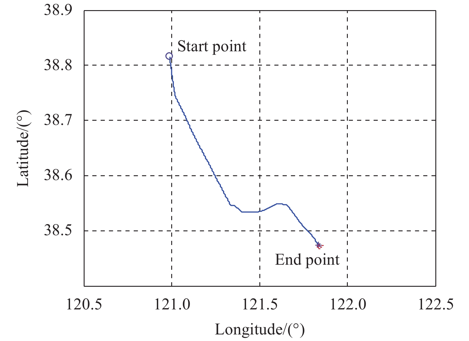
以某次航海试验数据为基础对所提方法的可行性及精度进行仿真分析。试验轨迹如图2所示。从图中可以看出,试验过程中有两次明显转弯,根据可观性分析,转弯有助于相关标定参数的收敛。

图 2 仿真用标定试验轨迹
Figure 2. Trajectory of calibration experiment in simulation
试验中使用的惯导为一90型捷联激光惯导,双频卫导接收机作为位置、速度输出设备。试验中所用惯导及卫导精度如表1所示。
表 1 仿真试验设备精度
Table 1. Specification of experimental devices
Accuracy Gyroscope/(°)·h-1 0.003 Accelerometer/mGal 50 GNSS position/m 3 GNSS velocity/m·s−1 0.03 由于该次海试试验未搭载里程仪,里程仪速度通过将卫导在n系下的速度投影到b系下而仿真生成。初始标定参数设置如表2所示。
表 2 初始标定参数设置
Table 2. Initial calibration parameter
Error Noise Scale factor error 0.03 0.01 Installation error/(°) 1 0.01 Current velocity/m·s−1 0.5 0.01 -
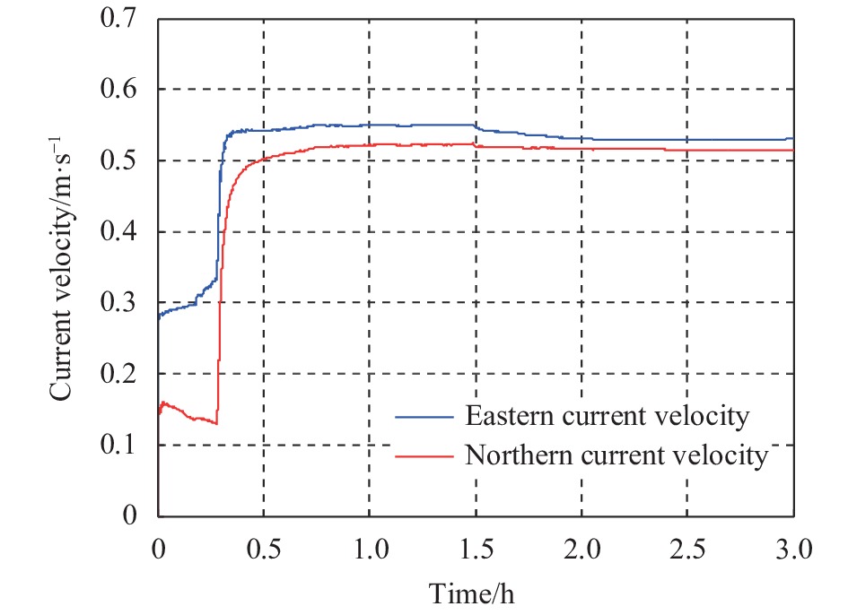
利用文中的方法对激光惯导/里程仪组合导航系统的参数进行标定。采用了多次标定法,其中第一次滤波后的结果如图3~图5所示。

图 3 一次滤波后的洋流速度估计结果
Figure 3. Current velocity estimation after first filtering

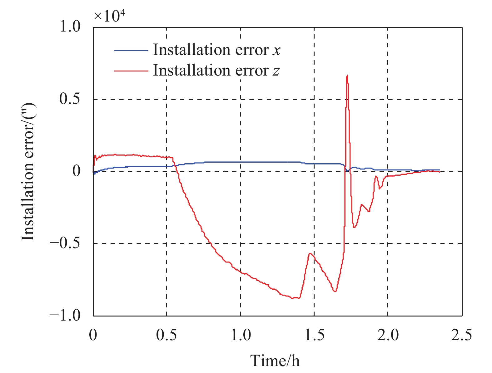
图 4 一次滤波后的安装误差角估计结果
Figure 4. Installation error estimation after first filtering

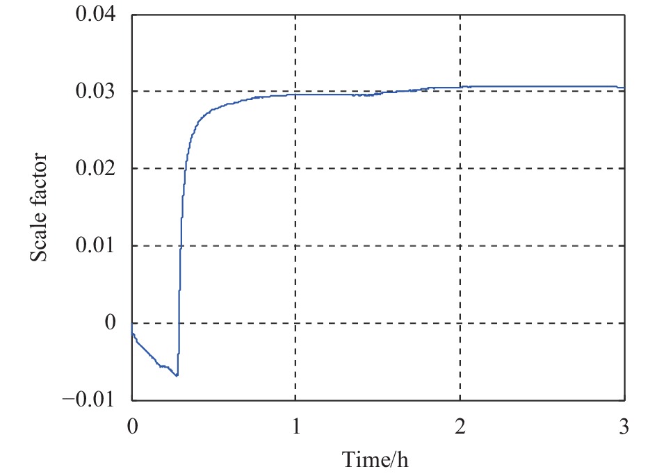
图 5 一次滤波后的比例因子误差估计结果
Figure 5. Scale factor estimation after first filtering
从图3~图5中可以看出,将洋流速度建模为状态量估计之后,经过一次滤波所有的标定参数都可以收敛到一个较为准确的值。而在1.5~2.2 h之间船经过两次转弯,可以看到标定参数收敛明显加快。
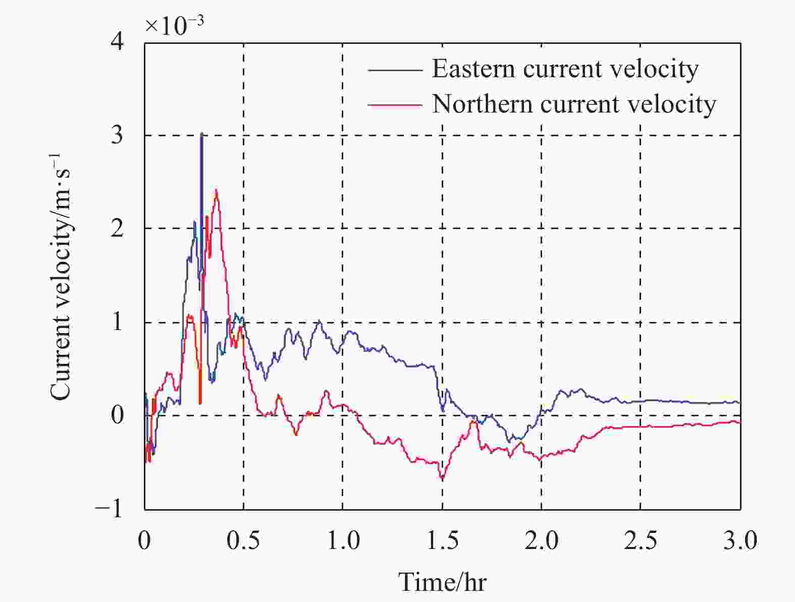
图 6 三次滤波后的洋流速度残差
Figure 6. Current velocity residual after third filtering
从图中可以看出,经过三次迭代滤波之后,标定参数基本收敛到真值,标定残差较小,洋流速度对标定参数的影响可以完全消除,验证了所提方法的有效性。
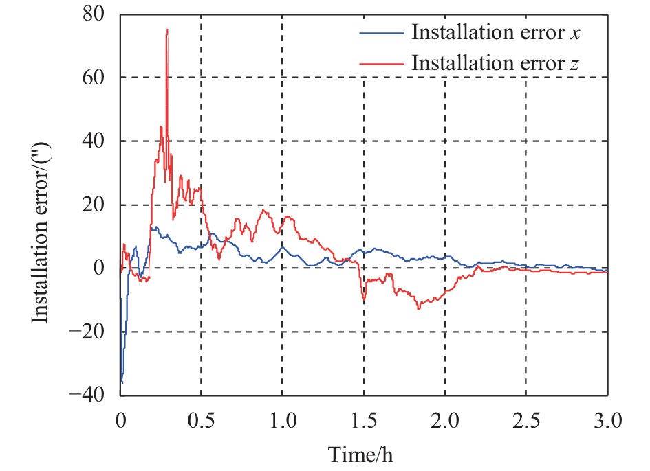
图 7 三次滤波后的安装误差估计残差
Figure 7. Installation error residual after third filtering
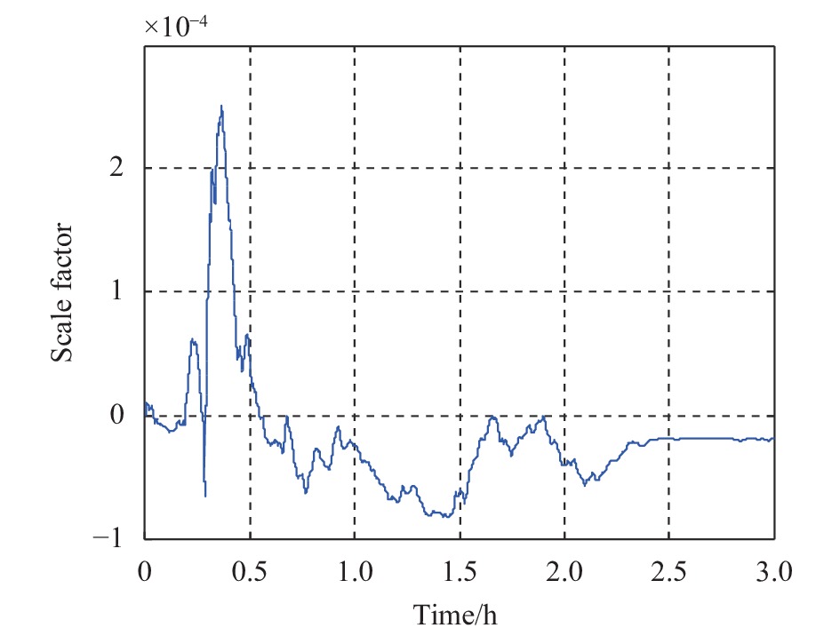
图 8 三次滤波后的比例因子估计残差
Figure 8. Scale factor residual after third filtering
-
以中国南海的某次海试为基础对文中的标定方法进行验证,试验中用到了50型激光陀螺捷联惯导以及电磁里程仪。卫导接收机输出作为速度及位置观测量。试验中所用设备的精度如表3所示。
表 3 里程仪海试试验设备精度
Table 3. Specification of experimental devices with EML
Accuracy Gyroscope/°/h 0.01 Accelerometer/mGal 100 GNSS position/m 3 GNSS velocity/m·s−1 0.03 EML/D 0.03 试验总时长9.4 h,取前面的2.4 h作为标定路径,如图9中小图所示。从图中可以看出,标定过程中有几次明显的转弯,根据可观性分析,转弯有助于提高相关参数的收敛速度,对于提高参数估计精度具有重要作用。经过多次迭代后,计算得到的标定结果如表4所示。
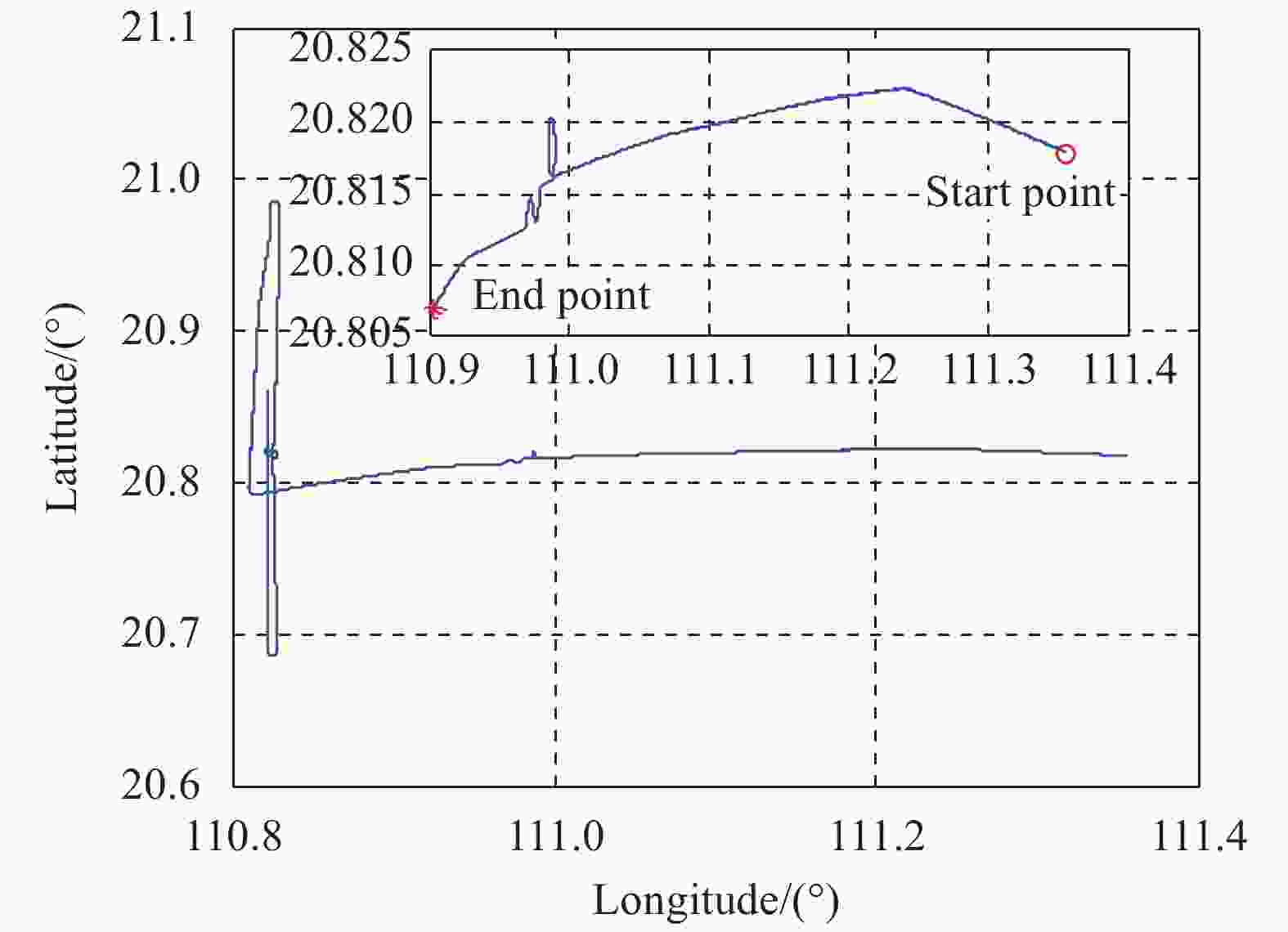
图 9 带里程仪的标定试验轨迹
Figure 9. Trajectory of calibration experiment with EML
表 4 标定结果
Table 4. Calibration result
Accuracy Scale factor −0.058 8 Installation error/(°) [−1.445 8, 0, 1.880 6] Current velocity/m·s−1 [1.092 0, 0.362 5] 相关参数的残差如图10、图11和图12所示。从图中可以看出,使用论文中的标定方法,经过多次迭代后,标定参数可以收敛到一个准确值,残差接近于0,相关参数的收敛速度也在转弯之后明显加快,与仿真结果类似。

图 10 带里程仪的海上洋流速度估计残差
Figure 10. Current velocity residual in the marine experiment with EML
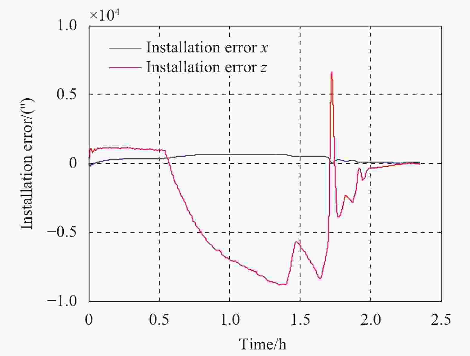
图 11 带里程仪的海上安装误差角估计残差
Figure 11. Installation error residual in the marine experiment with EML

图 12 带里程仪的海上比例因子估计残差
Figure 12. Scale factor residual in the marine experiment with EML
-
通过海试组合导航数据进一步验证标定参数的准确性,利用上节标定出的参数对里程仪及激光惯导之间的误差参数进行校正。海试试验总时长为9.4 h,试验轨迹如图9中的大图所示。图13所示为误差参数标定与未标定时的水平位置误差对比。

图 13 有无标定的海上水平位置误差试验结果对比
Figure 13. Position error comparison between with and without calibration in the marine experiment
从图中可以看出,标定参数补偿之后,水平误差得到了显著抑制,水平定位精度有了显著提升。试验结果证明了标定参数的准确性以及标定方法的可行性。
-
目前,船载测速设备主要基于分立式标定,分立式标定对海域、航行条件等要求较高。文中基于Kalman滤波方法设计了里程仪标定模型,将洋流速度建模为滤波状态量进行估计,有效避免了洋流速度对标定参数的影响。基于可观测性分析理论,分析了不同误差之间的耦合关系以及洋流速度的可观性,并据此设计了误差参数标定路径。试验结果表明,经过转弯之后洋流速度完全可观,其对其他参数的影响可以完全消除,验证了文中方法的有效性。
Calibration of RLG-INS/EML integrated navigation system considering current velocity
-
摘要: 在船载试验环境中,电磁里程仪的速度会受到洋流速度的影响。对于激光惯导/里程仪组合导航系统,洋流速度的存在会影响组合导航系统相关参数的标定。为克服洋流速度对标定结果的影响,论文在原有标定参数基础上将洋流速度建模为额外Kalman滤波状态量,并采用GNSS位置、速度信息作为滤波观测量来对参数进行估计。文中从里程仪的标定观测方程出发,分析了洋流速度对里程仪比例因子、安装误差角等误差参数标定结果的影响,以及不同误差参数之间的耦合关系;基于可观性分析理论研究了洋流速度及相关参数的可观测性,并确定了适用于洋流速度估计的标定路径。仿真及试验结果表明,经过几次转弯机动之后,包括洋流速度在内的所有标定参数均可收敛到一个准确值,有效解决了洋流速度对其他标定参数的影响。海试试验验证了文中方法的可行性。Abstract:
Objective The velocity output of an electromagnetic log (EML) is actually a velocity relative to the water. The current velocity will affect the velocity output of an EML in marine applications. If a ring laser gyroscope inertial navigation system (RLG-INS) is integrated with an EML to construct an integrated navigation system, the current velocity will produce negative effects on the calculation of calibration parameters, which thus leads to a degraded navigation performance in the following navigation process. In order to reduce the current velocity's effect on the calibration of a RLG-INS/EML integrated navigation system and improve the calibration accuracy of the relevant parameters, a calibration method of considering the current velocity effect is introduced. Methods Based on the integrated navigation principle, the current velocity can be augmented as an extra state in the calibration Kalman filter, while the GNSS position and velocity outputs are implemented as the Kalman filter's measurements to estimate these calibration parameters. The proposed method is beneficial in improving the calibration accuracy while estimating the current velocity concurrently. In such a case, the states estimated in the Kalman filter include attitude error, velocity error in eastern, northern and up directions, position error (longitude, latitude and height), gyroscope biases (three directions), accelerometer biases (three directions), installation error, scale factor error and current velocity in eastern and northern directions. Based on the calibration function, the effects of the current velocity on the EML scale factor and installation error are analyzed, which also reveals the coupling relationship among different calibration parameters. It is indicated that the attitude error related terms can be eliminated from the calibration equation especially when the attitude error is very large at the beginning of the navigation Kalman filter, which may cause a negative effect on the parameter estimation. An analysis of the current velocity's observability is also conducted, which is helpful in determining a proper calibration path to estimate the relevant states. Based on this observability analysis, a turn can help speed up the current velocity convergence. Therefore, it is suggested that some turns should be conducted during the calibration process. Results and Discussions The proposed method is further examined through the simulation and experiment. In the simulation, due to the absence of the EML, the EML velocity output is generated by converting the GNSS velocity in the navigation frame to the EML frame based on a real ship trajectory (Fig.2), while some errors such as scale factor error and installation error are also added to the generated simulation data. The simulation result indicates that the calibration parameters' residues can be reduced to a very small quantity after three iterations (Fig.3-8), if there are several turns in the trajectory. In the experiment, an EML and an INS are mounted together in a ship. The total experiment period is about 9.4 h, while the first 2.4 h are utilized to calibrate these parameters (Fig.9). All the parameters can be well estimated after 3 iterations and several turns, which verifies the effectiveness of the proposed method (Fig.10-12). The whole experiment period is used to examine the correctness of the calibration parameters. Compared with the result without calibration, the navigation performance can be greatly improved with the proposed calibration method (Fig.13). The maximum position drift is much smaller than the case without calibration. Conclusion The calibration of RLG-INS/EML integrated navigation system is very important in maintaining the navigation performance. Due to the effect of the current velocity, the calibration parameters will be polluted by this extra velocity. In this manuscript, a calibration method of considering the current velocity effect in proposed. The current velocity is augmented as an extra state in the calibration Kalman filter. The coupling relationship among different parameters is analyzed in theory, while a calibration strategy of improving the observability is also introduced. The simulation and experiment results verify the effectiveness of the proposed method. The proposed method can simplify the calibration process, which has potential in improving the calibration efficiency while maintaining the calibration accuracy. -
Key words:
- ring laser gyroscope INS /
- electromagnetic log /
- current velocity /
- parameter calibration
-
图 10 带里程仪的海上洋流速度估计残差
Figure 10. Current velocity residual in the marine experiment with EML
图 11 带里程仪的海上安装误差角估计残差
Figure 11. Installation error residual in the marine experiment with EML
图 12 带里程仪的海上比例因子估计残差
Figure 12. Scale factor residual in the marine experiment with EML
图 13 有无标定的海上水平位置误差试验结果对比
Figure 13. Position error comparison between with and without calibration in the marine experiment
表 1 仿真试验设备精度
Table 1. Specification of experimental devices
Accuracy Gyroscope/(°)·h-1 0.003 Accelerometer/mGal 50 GNSS position/m 3 GNSS velocity/m·s−1 0.03  下载: 导出CSV
表 2 初始标定参数设置
Table 2. Initial calibration parameter
Error Noise Scale factor error 0.03 0.01 Installation error/(°) 1 0.01 Current velocity/m·s−1 0.5 0.01
下载: 导出CSV
表 3 里程仪海试试验设备精度
Table 3. Specification of experimental devices with EML
Accuracy Gyroscope/°/h 0.01 Accelerometer/mGal 100 GNSS position/m 3 GNSS velocity/m·s−1 0.03 EML/D 0.03
下载: 导出CSV
表 4 标定结果
Table 4. Calibration result
Accuracy Scale factor −0.058 8 Installation error/(°) [−1.445 8, 0, 1.880 6] Current velocity/m·s−1 [1.092 0, 0.362 5]
下载: 导出CSV
-
[1] 顾鹏飞, 王省书, 郑佳兴, 等. 阻尼比连续可调的捷联惯性姿态测量系统内阻尼技术[J]. 红外与激光工程, 2017, 46(5): 122-128. doi: 10.3788/IRLA201746.0517004 Gu Pengfei, Wang Xingshu, Zheng Jiaxing, et al. Internal horizontal damping network of SAMS by applying adaptively adjustable damping ratio [J]. Infrared and Laser Engineering, 2017, 46(5): 0517004. (in Chinese) doi: 10.3788/IRLA201746.0517004 [2] 时海涛, 马静, 张小跃, 等. 里程计初始标定及误差分析[J]. 导航与控制, 2015, 14(5): 111-115. doi: 10.3969/j.issn.1674-5558.2015.05.020 Shi Haitao, Ma Jing, Zhang Xiaoyue, et al. The initial calibration of odometer and error analysis [J]. Navigation and Control, 2015, 14(5): 111-115. (in Chinese) doi: 10.3969/j.issn.1674-5558.2015.05.020 [3] 王琦, 高春峰, 周健, 等. 陆用组合导航中Janus 配置的激光多普勒测速仪的标定方法[J]. 红外与激光工程, 2019, 48(4): 248-254. doi: 10.3788/IRLA201948.0417003 Wang Qi, Gao Chunfeng, Zhou Jian, et al. Calibration method of laser Doppler velocimeter based on Janus configuration in land integrated navigation [J]. Infrared and Laser Engineering, 2019, 48(4): 0417003. (in Chinese) doi: 10.3788/IRLA201948.0417003 [4] 王琦, 高春峰, 聂晓明, 等. 陆用组合导航中二维激光多普勒测速仪的标定方法[J]. 中国激光, 2018, 45(8): 151-157. Wang Qi, Gao Chunfeng, Nie Xiaoming, et al. Calibration method of two-dimensional laser Doppler velocimeter in land integrated navigation system [J]. Chinese Journal of Lasers, 2018, 45(8): 0804004. (in Chinese) [5] Xu Xiang, Gui Jing, Sun Yifan, et al. A robust in-motion alignment method with inertial sensors and doppler velocity log [J]. IEEE Transactions on Instrumentation and Measurement, 2021, 70: 8500413. doi: 10.1109/TIM.2020.3011873 [6] Ben Yueyang, Zang Xinle, Sun Yifan, et al. A dual-state filter for a relative velocity aiding strapdown inertial navigation system [J]. IEEE Transactions on Instrumentation and Measurement, 2021, 70: 1000215. doi: 10.1109/TIM.2020.3010042 [7] Yao Yiqing, Xu Xiaosu, Hou Lanhua, et al. A simple and precise correction method for DVL measurements under the dynamic environment [J]. IEEE Transactions on Vehicular Technology, 2020, 69(10): 10750-10758. doi: 10.1109/TVT.2020.3008755 [8] Zhao Liye, Liu Xianjun, Wang Lei, et al. A pretreatment method for the velocity of DVL based on the motion constraint for the integrated SINS/DVL [J]. Applied Sciences, 2016, 6(3): 79-93. doi: 10.3390/app6030079 [9] Song Zhuoyuan, Mohseni Kamran. Long-term inertial navigation aided by dynamics of flow field features [J]. IEEE Journal of Oceanic Engineering, 2018, 43(4): 940-954. doi: 10.1109/JOE.2017.2766900 [10] 吕志刚. 基于SINS/DVL/GPS的AUV组合导航标定方法的研究及其误差分析[J]. 舰船电子工程, 2018, 38(6): 33-36. doi: 10.3969/j.issn.1672-9730.2018.01.009 Lv Zhigang. Research on SINS/DVL/GPS integrated navigation system calibration method and the error analysis of AUV [J]. Ship Electronic Engineering, 2018, 51(1): 33-36. (in Chinese) doi: 10.3969/j.issn.1672-9730.2018.01.009 [11] 白龙, 张淏酥, 吴爽, 等. AUV组合导航系统的DVL标定方法研究 [J]. 舰船电子工程, 2021, 41(11): 46-53. doi: 10.3969/j.issn.1672-9730.2021.11.011 Bai Long, Zhang Haosu, Wu Shuang, et al. Research on DVL calibration method of AUV integrated navigation system [J]. Ship Electronic Engineering, 2021, 41(11): 46-53. (in Chinese) doi: 10.3969/j.issn.1672-9730.2021.11.011 [12] 李志炜, 岳崴, 高胜峰, 等. 基于可观测度反馈的SINS/DVL组合导航算法 [J]. 舰船电子工程, 2020, 28(2): 155-161. Li Zhiwei, Yue Wei, Gao Shengfeng, et al. The SINS/DVL integrated navigation algorithm based on observable degree feedback [J]. Journal of Unmanned Undersea Systems, 2020, 28(2): 155-161. (in Chinese) [13] Liu Peijia, Wang Bo, Hou Dongdong, et al. An approach for DVL-aided SINS in-motion alignment based on observability analysis [J]. IEEE Sensors Journal, 2021, 21(15): 17131-17143. doi: 10.1109/JSEN.2021.3081865 [14] Medagoda Lashika, Kinsey James C, Eilders Martin. Autonomous underwater vehicle localization in a spatiotemporally varying water current field [C]//Proc of IEEE International Conference on Robotics and Automation (ICRA), 2015: 565-572. [15] Liu Peijia, Wang Bo, Deng Zhihong, et al. INS/DVL/PS tightly-coupled underwater navigation method with limited DVL measurements [J]. IEEE Sensors Journal, 2018, 18(7): 2994-3002. doi: 10.1109/JSEN.2018.2800165 [16] Hegrenæs Øyvind, Berglun Einar. Doppler water-track aided inertial navigation for autonomous underwater vehicle [C]// OCEANS 2009-EUROPE, 2009: 1-10. [17] Liu Xianjun, Liu Xixiang, Wang Lei, et al. SINS/DVL integrated system with current and misalignment estimation for midwater navigation [J]. IEEE Access, 2021, 9: 51332-51342. doi: 10.1109/ACCESS.2021.3069469 [18] Chang Lubin. Robust initial attitude alignment for SINS/DVL [J]. IEEE/ASME Transactions on Mechatronics, 2018, 23(4): 2016-2021. doi: 10.1109/TMECH.2018.2834917 -

 点击查看大图

计量
- 文章访问数: 144
- HTML全文浏览量: 31
- PDF下载量: 19
- 被引次数: 0

